Further topics on r.v.
Derived distributions
Probability law on \(Y\), where \(Y=g(X)\) depends on whether \(X\) is discrete or continuous r.v.. In the first case, our computations are based on the fact that \(p_Y(y)=\mathbb P(g(X)=y)\). Else, we follow a two-step procedure: find \(F_Y(y)=\mathbb P(g(X)\le y)\), and differentiate \(f_Y(y)=\frac{\partial}{\partial y}F_Y(y)\).
| \(g(X)\) | \(X\) discrete | \(X\) continuous |
|---|---|---|
| linear \(g(X)=aX+b\) |
\(\displaystyle p_Y(y)=p_X\left(\frac{y-b}{a}\right)\) | \(\displaystyle f_Y(y)=f_X\left(\frac{y-b}{a}\right)\frac{1}{\lvert a\rvert}\) |
| strictly monotonic (hence invertible) \(X=h(Y)\) |
\(\displaystyle p_Y(y)=p_X(h(y))\) | \(\displaystyle f_Y(y)=f_X(h(y))\left\lvert\frac{\partial}{\partial y}h(y)\right\rvert\) |
| general | \(\displaystyle p_Y(y)=\sum_{x:g(x)=y}p_X(x)\) | \(\displaystyle f_Y(y)=\sum_{h_i(y):g(h_i(y))=y}f_X(h_i(y))\left\lvert\frac{\partial}{\partial y}h_i(y)\right\rvert\) |
Note that if \(X\) is uniform (irrespective if discrete or continuous), a linear combination \(Y=aX+b\) is still uniform, just with a different scale and location.
The general continuous case assumes that the domain can be split into intervals within which \(g(X)\) is still strictly monotonic, this to ensure that \(\nexists y:\mathbb P(Y=y)\neq0\). Otherwise, we would fall into a mixed discrete/continuous r.v. case.
Finally, if \(X\sim\mathcal N(\mu_X,\sigma_X^2)\) then for any \(Y=aX+b\), we have that \(Y\sim\mathcal N(a\mu_X+b,a^2\sigma_X^2)\).
Simulation
Assume \(U=F_X(X)\) with \(F_X\) invertible. To compute CDF of \(U\), we can rely on the above and derive \(F_U(u)=\mathbb P(U\le u)=\mathbb P(F_X(X)\le u)=\mathbb P(X\le F_X^{-1}(u))=F_X(F_X^{-1}(u))=u\). Recall that the only r.v. that satisfies this CDF is \(\text{Unif}([0,1])\). In addition, this also means that if \(U_i\overset{\text{i.i.d.}}{\sim}\text{Unif}([0,1])\), then \(F_X(U_i)\overset{\text{i.i.d.}}{\sim}X\). This allows us to conclude an approach to simulate any distribution, depending on whether \(X\) is discrete or continuous.
- \(X\) discrete r.v.: we assign to \(X\) the \(k\)-th value that satisfies \(F_X(k-1)\lt u\le F_X(k)\); and
- \(X\) continuous r.v.: we assign to \(X\) that \(x\) that satisfies \(u=F_X(x)\).
Function of multiple r.v.
Calculating probability law on \(Z=g(X,Y)\) is not different from the single r.v. case. If \(f_{Y\lvert X}(y\lvert x)\) is available and \(\exists h:Y=h(Z,X)\), we can compute \(f_{Z\lvert X}(z\lvert x)\) in terms of \(f_{Y\lvert X}(y\lvert x)\) and \(y=h(z,x)\) bearing in mind that \(X=x\) is given. In other words, we derive \(F_{Z\lvert X}(z\lvert x)=F_{Y\lvert X}(h(x,z)\lvert x)\), and then differentiate \(f_{Z\lvert X}(z\lvert x)=f_{Y\lvert X}(h(x,z)\lvert x)\left\lvert\frac{\partial}{\partial z}h(x,z)\right\rvert\). At this point, total probability theorem tells us that \(f_Z(z)=\int_{-\infty}^\infty f_X(x)f_{Z\lvert X}(z\lvert x)dx\).
Sometimes, calculations can be simplified. Assume \(f_{X,Y}(x,y)=c\) is constant and \(Z=g(X,Y)\) is associated with area \(A(Z)\) in the \(X\)—\(Y\) plane. In this case, \(F_Z(z)=\mathbb P(g(X,Y)\le z)=cA(z)\).
As for \(\max\) and \(\min\) functions, if \(X\ind Y\), we have \(\mathbb P(\max\{X,Y\}\le z)=F_X(z)F_Y(z)\), and \(\mathbb P(\min\{X,Y\}\le z)=1-(1-F_X(z))(1-F_Y(z))\).
Sum of independent r.v.
If \(X\) and \(Y\) are discrete r.v., with \(X\ind Y\), the distribution of \(Z=X+Y\) can be obtained by deriving \(p_{Z\lvert X}(z\lvert x)=p_Y(z-x)\) and computing \(p_Z(z)=\sum_x p_X(x)p_Y(z-x)\). If \(X\) and \(Y\) are continuous, use \(f_{Z\lvert X}(z\lvert x)=f_Y(z-x)\) and \(f_Z(z)=\int_{-\infty}^\infty f_X(x)f_Y(z-x)dx\) instead. Due to its widespread use, the aforementioned formula is referred to as convolution.
For the general case \(Z=aX+bY\), where \(a,b\in\mathbb R\), we get either \(p_Z(z)=\sum_x p_X(\frac{x}{a})p_Y(\frac{z-x}{b})\) or \(f_Z(z)=\int_{-\infty}^\infty f_X(\frac{x}{a})\frac{1}{\lvert a\rvert}f_Y(\frac{z-x}{b})\frac{1}{\lvert b\rvert}dx\), depending on whether \(X\) and \(Y\) are discrete or continuous.
Sum of independent Normal r.v.
If \(X\sim\mathcal N(\mu_X,\sigma_X^2)\), \(Y\sim\mathcal N(\mu_Y,\sigma_Y^2)\), and \(X\ind Y\), expectation and variance of \(Z=X+Y\) are \(\mu_Z=\mathbb E[Z]=\mu_X+\mu_Y\) and \(\sigma_Z^2=\text{var}(X+Y)=\sigma_X^2+\sigma_Y^2\), respectively. Also, the distribution of \(Z\) is normal as well, with \(Z\sim\mathcal N(\mu_Z,\sigma_Z^2)\).
To prove the Normality of \(Z\), consider \(f_Z(z)=\int_{-\infty}^\infty f_X(x)f_Y(z-x)dx\) as in the previous segment and observe that the joint PDF can be rewritten as \(f_X(x)f_Y(z-x)=f_Z(z)f_{X\lvert Z}(x\lvert z)\) thanks to some reshuffling of the terms, where \(\mu_{X\lvert Z}=\frac{\mu_X\sigma_Y^2+(z-\mu_Y)\sigma_X^2}{\sigma_X^2+\sigma_Y^2}\) and \(\sigma_{X\lvert Z}^2=\frac{\sigma_X^2\sigma_Y^2}{\sigma_X^2+\sigma_Y^2}\),leading to the following.
\[\begin{align} f_Z(z) &=\int_{-\infty}^\infty\frac1{\sqrt{2\pi\sigma_Z^2}}\exp\left\{-\frac12\left(\frac{z-\mu_Z}{\sigma_Z}\right)^2\right\}\frac{1}{\sqrt{2\pi\sigma_{X\lvert Z}^2}}\exp\left\{-\frac12\left(\frac{x-\mu_{X\lvert Z}}{\sigma_{X\lvert Z}}\right)^2\right\}dx\\ &=\frac{1}{\sqrt{2\pi\sigma_Z^2}}\exp\left\{-\frac12\left(\frac{z-\mu_Z}{\sigma_Z}\right)^2\right\}\cancelto{=1}{\int_{-\infty}^\infty\frac{1}{\sqrt{2\pi\sigma_{X\lvert Z}^2}}\exp\left\{-\frac12\left(\frac{x-\mu_{X\lvert Z}}{\sigma_{X\lvert Z}}\right)^2\right\}dx} \end{align}\]Covariance
Defined as \(\sigma_{XY}=\text{cov}(X,Y)=\mathbb E[(X-\mathbb E[X])(Y-\mathbb E[Y])]\), covariance is a measure of the joint variability of two r.v..
| Property | Formula |
|---|---|
| Variance | \(\text{cov}(X,X)=\text{var}(X)\) |
| Symmetry | \(\text{cov}(X,Y)=\text{cov}(Y,X)\) |
| Independence | \(\text{cov}(X,a)=0\), for any \(a\) constant \(X\ind Y\implies\text{cov}(X,Y)=0\) (the converse is not true in general) |
| Bilinear | \(\text{cov}(aX,bY+cZ)=ab\cdot\text{cov}(X,Y)+ac\cdot\text{cov}(X,Z)\) |
| Variance | \(\displaystyle\text{var}\left(\sum_{i=1}^n a_iX_i\right)=\underbrace{\sum_{i=1}^n a_i^2\text{var}(X_i)}_{\text{$n$ terms}}+\underbrace{\sum_{i\neq j}a_ia_j\text{cov}(X_i,X_j)}_{\text{$n^2-n$ terms}}\) \(\text{var}(aX+bY)=a^2\text{var}(X)+b^2\text{var}(Y)+2ab\text{cov}(X,Y)\) |
| Equivalency | \(\begin{align}\text{cov}(X,Y)&=\mathbb E[XY]-\mathbb E[X]\mathbb E[Y]\\&=\mathbb E[(X-\mathbb E[X])Y]\\&=\mathbb E[\mathbb E[XY\lvert X]]-\mathbb E[X]\mathbb E[\mathbb E[Y\lvert X]]\end{align}\) |
Assume \(A=X+Y\) and \(B=X-Y\) and \(\sigma_X^2=\sigma_Y^2\). \(A\) and \(B\) are not independent, since they are both linear combinations of \(X\) and \(Y\); at the same time \(\sigma_{AB}=\text{cov}(A,B)=\sigma_X^2-\sigma_Y^2=0\) and therefore \(\sigma_{AB}=0\) does not imply \(A\ind B\).
Covariance matrix
Assume a random vector \(\mathbf X=\begin{bmatrix}X_1,\dots,X_d\end{bmatrix}^T\in\mathbb R^d\), where every entry \(X_i\) is a r.v. A covariance matrix is defined as \(\Sigma_{\mathbf X}=\text{cov}(\mathbf X)=\mathbb E[(\mathbf X-\mu_{\mathbf X})(\mathbf X-\mu_{\mathbf X})^T]\), where \(\mu_{\mathbf X}=\mathbb E[\mathbf X]\), which will have the following form.
\[(\Sigma_\mathbf X)_{ij}=\begin{cases} \text{var}(X_i)&i=j\\ \text{cov}(X_i,X_j)&i\neq j \end{cases}\]| Property | Formula |
|---|---|
| Symmetry | \(\Sigma_{\mathbf X}=\Sigma_{\mathbf X}^T\) |
| Eigen-decomposition (diagonalization) | \(\mathbf P^T\Sigma_{\mathbf X}\mathbf P=\mathbf D\), where \(\mathbf P\) orthogonal (\(\mathbf P^T\mathbf P=\mathbf P\mathbf P^T=\mathbf I\)), and \(\mathbf D\) diagonal matrix formed with eigenvalues of \(\Sigma_{\mathbf X}\) |
| Semi-positive definite | \(\mathbf x^T\Sigma_{\mathbf X}\mathbf x\ge0\), \(\forall\mathbf x\in\mathbb R^d\). If \(\mathbf x^T\Sigma_{\mathbf X}\mathbf x=0\) for some \(\mathbf x\), then \(\Sigma_{\mathbf X}\) is not invertible, and \(\Sigma_{\mathbf X}^{-1}\) does not exist |
| Square root | \(\exists!\Sigma_{\mathbf X}^{\frac 1 2}\) semi-positive definite, s.t. \(\Sigma_{\mathbf X}^{\frac 1 2}\Sigma_{\mathbf X}^{\frac 1 2}=\Sigma_{\mathbf X}\) |
| Scaled by the square | \(\text{cov}(\mathbf A^T\mathbf X)=\mathbf A^T\Sigma_{\mathbf X}\mathbf A\) |
| Invariant with respect to location | \(\text{cov}(\mathbf A^T\mathbf X+\mathbf B)=\mathbf A^T\Sigma_{\mathbf X}\mathbf A\) |
Correlation
Correlation is a measure of the degree of linear association, whether causal or not, between two r.v. and is defined as \(\rho_{XY}=\mathbb E\left[\left(\frac{X-\mathbb E[X]}{\sigma_X}\right)\left(\frac{Y-\mathbb E[Y]}{\sigma_Y}\right)\right]=\frac{\text{cov}(X,Y)}{\sigma_X\sigma_Y}\).
Main properties of the correlation coefficient are that \(\lvert\rho\rvert\le1\) and that \(\lvert\rho\rvert=1\implies Y=aX\), with \(a\) constant, while others can be derived directly from covariance.
Bivariate Normal r.v.
Normal r.v. \(X\) and \(Y\) are said to be jointly bivariate Normal if \(aX+bY\) is Normal for any \(a,b\in\mathbb R\). From this statement, once can conclude that:
- if \(a=1\) and \(b=0\), then \(X\sim\mathcal N(\mu_X,\sigma_X^2)\) has to be Normal;
- if \(a=0\) and \(b=1\), then \(Y\sim\mathcal N(\mu_Y,\sigma_Y^2)\) has to be Normal; and
- if \(a=b=1\), then \(X+Y\sim\mathcal N(\mu_X+\mu_Y,\sigma_X^2+\sigma_Y^2+2\sigma_{XY})\).
To derive the joint PDF, one could split \(f_{XY}(x,y)=f_X(x)f_{Y\lvert X}(y\lvert x)\), and find \(Y\lvert X\) that would satisfy the above relations. Long story short, it turns out that if \(X\) and \(Y\) are bivariate Normal, then there exist \(Z_1,Z_2\overset{\text{i.i.d.}}{\sim}\mathcal N(0,1)\) s.t.
\[\begin{cases} X=\mu_X+\sigma_XZ_1\\ Y=\mu_Y+\sigma_Y\left(Z_1\rho_{XY}+Z_2\sqrt{1-\rho_{XY}^2}\right) \end{cases}\]Now, since \(Z_1\lvert X=\frac{x-\mu_X}{\sigma_X}\), if follows that \(Y\lvert X\sim\mathcal N(\mu_{Y\lvert X},\sigma_{Y\lvert X}^2)\), with the following parameters.
\[\begin{cases} \displaystyle\mu_{Y\lvert X}=\mathbb E\left[\left.\mu_Y+\sigma_Y\left(\frac{x-\mu_X}{\sigma_X}\rho_{XY}+Z_2\sqrt{1-\rho_{XY}^2}\right)\right\rvert X\right]=\mu_Y+\rho_{XY}\frac{\sigma_Y}{\sigma_X}(x-\mu_X)\\ \displaystyle\sigma_{Y\lvert X}^2=\text{var}\left(\left.\mu_Y+\sigma_Y\left(\frac{x-\mu_X}{\sigma_X}\rho_{XY}+Z_2\sqrt{1-\rho_{XY}^2}\right)\right\rvert X\right)=\sigma_Y^2(1-\rho_{XY}^2) \end{cases}\]Putting together all the pieces, the joint PDF takes the following form.
\[\begin{align} f_{XY}(x,y) &=f_X(x)f_{Y\lvert X}(y\lvert x)\\ &=\frac1{\sqrt{2\pi\sigma_X^2}}\exp\left\{-\frac12\left(\frac{x-\mu_X}{\sigma_X}\right)^2\right\}\frac1{\sqrt{2\pi\sigma_{Y\lvert X}^2}}\exp\left\{-\frac12\left(\frac{y-\mu_{Y\lvert X}}{\sigma_{Y\lvert X}}\right)^2\right\}\\ &=\frac1{\sqrt{(2\pi)^2\sigma_X^2\sigma_{Y\lvert X}^2}}\exp\left\{-\frac12\left[\left(\frac{x-\mu_X}{\sigma_X}\right)^2+\left(\frac{y-\mu_{Y\lvert X}}{\sigma_{Y\lvert X}}\right)^2\right]\right\}\\ \end{align}\]Finally, replacing \(\mu_{Y\lvert X}=\mu_Y+\rho_{XY}\frac{\sigma_Y}{\sigma_X}(x-\mu_X)\) and \(\sigma_{Y\lvert X}^2=\sigma_Y^2(1-\rho_{XY}^2)\), we conclude that to satisfy the initial condition above, the joint PDF \(f_{XY}(x,y)\) must have the following form.
\[\begin{align} &f_{XY}(x,y)=\frac1{\sqrt{(2\pi)^2\sigma_X^2\sigma_Y^2(1-\rho_{XY}^2)}}\times\\ &\times\exp\left\{-\frac{1}{2(1-\rho_{XY}^2)}\left[\left(\frac{x-\mu_X}{\sigma_X}\right)^2-2\rho_{XY}\left(\frac{x-\mu_X}{\sigma_X}\right)\left(\frac{y-\mu_Y}{\sigma_Y}\right)+\left(\frac{y-\mu_Y}{\sigma_Y}\right)^2\right]\right\} \end{align}\]Or, more compactly, \(f_\mathbf Z(\mathbf z)=\frac1{\sqrt{(2\pi)^2\det(\Sigma_\mathbf Z)}}\exp\left\{-\frac12(\mathbf z-\mu_\mathbf Z)^T\Sigma_\mathbf Z^{-1}(\mathbf z-\mu_\mathbf Z)\right\}\).
\[\begin{align} \mathbf z=\begin{bmatrix}x\\y\end{bmatrix}&&\mu_\mathbf Z=\begin{bmatrix}\mu_X\\\mu_Y\end{bmatrix}&&\Sigma_\mathbf Z=\begin{bmatrix}\sigma_X^2&\rho_{XY}\sigma_X\sigma_Y\\\rho_{XY}\sigma_X\sigma_Y&\sigma_Y^2\end{bmatrix} \end{align}\]Prior to concluding, an important observation is that \(f_{XY}(x,y)=f_X(x)f_Y(y)\) when \(\rho_{XY}=0\). This means that if \(X\) and \(Y\) are jointly Normal and uncorrelated, then they are also independent.
Multivariate Normal r.v.
A random vector \(\mathbf X\in\mathbb R^d\) is a multivariate Normal r.v., and is defined as \(\mathbf X\sim\mathcal N_d(\mu_\mathbf X,\Sigma_\mathbf X)\) if \(\forall\mathbf A\in\mathbb R^d\), we have that \(\mathbf A^T\mathbf X\sim\mathcal N_d\left(\mathbf A^T\mu_\mathbf X,\mathbf A^T\Sigma_\mathbf X\mathbf A\right)\).
If the above condition holds, then the PDF of \(\mathbf X\) is as follows.
\[f_\mathbf X(\mathbf x)=\frac 1 {\sqrt{(2\pi)^d\det(\Sigma_\mathbf X)}}\exp\left\{-\frac 1 2(\mathbf x-\mu_\mathbf X)^T\Sigma_\mathbf X^{-1}(\mathbf x-\mu_\mathbf X)\right\}\]Above definition implies that any linear combination of elements of \(\mathbf X\) is one-dimension Normal r.v. (or a constant, that is a Normal r.v. with zero variance), which in turn requires every \(X_i\) to be Normal r.v. and any pair \((X_i,X_j)\) to be a bivariate Normal r.v..
The latter condition should not be taken for granted. Assume \(X_i\sim\mathcal N(0,1)\) and \(X_j=RX_i\), where \(R\sim\href{/2022/01/08/discrete-random-variables.html#basic}{\text{Rad}}\). In this case, despite both \(X_i\) and \(X_j\) are standard Normal r.v., their sum is not a Normal r.v.
\[X_i+X_j=\begin{cases}0&\text{with probability $\frac 1 2$}\\2X_i&\text{with probability $\frac 1 2$}\end{cases}\]Conversely, any bivariate Normal r.v. can be derived from multivariate Normal r.v. with \(d=2\). Assume \(Z_1,Z_2\overset{\text{i.i.d.}}{\sim}\mathcal N(0,1)\) and \(\mathbf Z=\begin{bmatrix}Z_1&Z_2\end{bmatrix}^T\). Note that any \(\mathbf X=\begin{bmatrix}X_1&X_2\end{bmatrix}\) with covariance \(\rho\sigma_1\sigma_2\)can be expressed as \(\mathbf X=\mathbf A^T\mathbf Z+\mu_{\mathbf X}\).
\[\mathbf A^T\mathbf Z+\mu_{\mathbf X}=\begin{bmatrix}\sigma_1&0\\\sigma_2\rho&\sigma_2\sqrt{1-\rho^2}\end{bmatrix}\begin{bmatrix}Z_1\\Z_2\end{bmatrix}+\begin{bmatrix}\mu_1\\\mu_2\end{bmatrix}=\begin{bmatrix}\sigma_1 Z_1+\mu_1\\\sigma_2(Z_1\rho+Z_2\sqrt{1-\rho^2})+\mu_2\end{bmatrix}\]In particular, if \(\mathbf Z\sim\mathcal N_2(\mathbf 0_2,\mathbf I_2)\), then \(\mathbf X\sim\mathcal N_2(\mu_\mathbf X,\Sigma_\mathbf X)\), where the covariance matrix is as follows.
\[\Sigma_\mathbf X=\mathbf A^T\mathbf A=\begin{bmatrix}\sigma_1&0\\\sigma_2\rho&\sigma_2\sqrt{1-\rho^2}\end{bmatrix}\begin{bmatrix}\sigma_1&\sigma_2\rho\\0&\sigma_2\sqrt{1-\rho^2}\end{bmatrix}=\begin{bmatrix}\sigma_1^2&\rho\sigma_1\sigma_2\\\rho\sigma_1\sigma_2&\sigma_2^2\end{bmatrix}\]Computing \(f_{X_1X_2}(x_1,x_2)\) as PDF of a bivariate Normal r.v. from direct application of the definition of \(f_\mathbf X(\mathbf x)\) should be straightforward. Prior to concluding, observe that standardization of \(\mathbf X\) can be obtained as \(\mathbf Z=\Sigma_{\mathbf X}^{-\frac 1 2}(\mathbf X-\mu_{\mathbf X})\), which with \(d=2\) becomes \(\mathbf Z=(\mathbf A^T)^{-1}(\mathbf X-\mu_{\mathbf X})\).
Total expectation and total variance
So far, we saw that for any r.v. \(X\), \(\mathbb E[X]\) is a number. Same thing happens with conditional expectation, as \(g(y)=\mathbb E[X\lvert Y=y]\) is still a number, which depends on parameter \(y\). However, since any function of a r.v. is a r.v. itself, it follows that \(g(Y)=\mathbb E[X\lvert Y]\) is a r.v., with its own distribution, expectation and variance. Same considerations apply to any other function \(\mathbb E[h(X)\lvert Y]\), such as \(\text{var}(X\lvert Y)=\mathbb E[(X-\mathbb E[X\lvert Y])^2\lvert Y]\), where the inner \(\mathbb E[X\lvert Y]\) reminds us that all expectations are conditional on \(Y\).
Assuming for simplicity discrete case, we observe that in accordance with the total expectation theorem we have that \(\mathbb E[\mathbb E[X\lvert Y]]=\sum_y p_Y(y)\mathbb E[X\lvert Y=y]=\mathbb E[X]\). This is known as the law of total expectation, also referred to as the law of iterated expectations.
Analogously, one can derive the following relation, known as the law of total variance.
\[\begin{align} \text{var}(X) &=\mathbb E[X^2]-(\mathbb E[X])^2=\mathbb E[\mathbb E[X^2\lvert Y]-(\mathbb E[\mathbb E[X\lvert Y]])^2\\ &=\underbrace{\mathbb E[\mathbb E[X^2\lvert Y]]{\color{red}-\mathbb E[(\mathbb E[X\lvert Y])^2]}}_{\mathbb E[\text{var}(X\lvert Y)]}\underbrace{ {\color{red}+\mathbb E[(\mathbb E[X\lvert Y])^2]}-(\mathbb E[\mathbb E[X\lvert Y]])^2}_{\text{var}(\mathbb E[X\lvert Y])}\\ &=\mathbb E[\text{var}(X\lvert Y)]+\text{var}(\mathbb E[X\lvert Y]) \end{align}\]The above is particularly useful to compute expectation and variance of a sum of \(N\) r.v., where \(N\) is in turn a r.v. Assume \(Y=\sum_{i=1}^N X_i\), with \(X_i\overset{\text{i.i.d.}}{\sim}\mathcal P\), and note that \(\mathbb E[Y]=\mathbb E[\mathbb E[Y\lvert N]]=\mathbb E[N\mathbb E[X_i]]\) and therefore \(\mathbb E[Y]=\mathbb E[N]\mathbb E[X_i]\). As for the variance, consider the above relationship and observe that \(\text{var}(Y)=\mathbb E[N\text{var}(X_i)]+\text{var}(N\mathbb E[X_i])=\mathbb E[N]\text{var}(X_i)+(\mathbb E[X_i])^2\text{var}(N)\).
Final remark is that \(\mathbb E[g(Y)X\lvert Y]=g(Y)\mathbb E[X\lvert Y]\), which comes from the observation that given \(Y=y\), \(g(Y)\) is a constant and can be pulled out of the expectation. Also, for any invertible function \(h(Y)\), we have that \(\mathbb E[X\lvert Y]=\mathbb E[X\lvert h(Y)]\), due to the fact that \(\mathbb P(Y\le y)=\mathbb P(h(Y)\le h(y))\).
Categorical distribution
Assume you have a r.v. \(X\) that can take on one of \(d\) possible categories. There is no innate underlying ordering of these outcomes, and sometimes numerical labels are often attached for convenience in describing the distribution, such as \(\{a_1,\dots,a_d\}\). For convenience, a multivariate r.v. \(\mathbf X\) is defined in the form \(\mathbf X=\begin{bmatrix}\mathbb 1(X=a_1)&\dots&\mathbb 1(X=a_d)\end{bmatrix}^T\). Individual probabilities \(p_i\) associated with each category \(j\) are collected in a parameter vector \(\mathbf p=\begin{bmatrix}p_1&\dots&p_d\end{bmatrix}^T\in\Delta_d\), where \(\Delta_d\subset\mathbb R^d\) is a probability simplex of dimension \(d\), defined as \(\Delta_d=\left\{\mathbf p\in\mathbb R^d:p_j\ge0,\sum_{j=1}^d p_j=1\right\}\).
Accordingly, \(\text{Cat}(\mathbf p)\) determines a Categorical distribution that is the most general distribution over a \(d\)-way event, where any other discrete distribution over a size \(d\) sample space is a special case. For example, \(\text{Ber}(p)=\text{Cat}(\begin{bmatrix}1-p&p\end{bmatrix}^T)\) and \(\text{Unif}(1,d)=\text{Cat}\left(\frac1d\mathbf 1_d\right)\), where we only need to specify the categories attached with the probabilities, such as \(\{0,1\}\) or \(\{1,\dots,d\}\) in the case of Bernoulli or Uniform distribution, respectively.
Categorical can also approximate discrete r.v. with infinite support, such as \(\text{Geom}(p)\) or \(\text{Pois}(\lambda)\), although it is clear that to describe completely these distributions, \(\mathbf p\) would be an infinite long vector, which is a clear example of non parametric statistics. The approximation can be done by taking a bin to hold all residual numbers, that could occur with extremely low probability.
Observe that due to its construction, when one element of \(\mathbf X\) is equal to \(1\) all others are necessarily \(0\). This means that elements of \(\mathbf X\) are not independent from each other. Accordingly, the associated covariance matrix is as follows.
\[\Sigma_{\mathbf X}=\begin{bmatrix}p_1(1-p_1)&&-p_1p_d\\&\ddots&\\-p_1p_d&&p_d(1-p_d)\end{bmatrix}\]| r.v. | PMF \(p_X(x)\) |
Expectation \(\mu_{\mathbf X}=\mathbb E[\mathbf X]\) |
Variance \(\Sigma_{\mathbf X}=\text{cov}(\mathbf X)\) |
|---|---|---|---|
| Categorical \(\text{Cat}(\mathbf p)\) |
\(\begin{cases}\prod_{j=1}^d p_j^{X_j}&\mathbf X\in\{0,1\}^d\\0&\text{otherwise}\end{cases}\) \(\mathbf 1_d^T\mathbf X=1\), \(\mathbf 1_d^T\mathbf p=1\) |
\(\mathbf p\) | \(\Sigma_\mathbf X\) |
| Multinomial \(\text{Mult}(k,\mathbf p)\) |
\(\begin{cases}{k\choose\mathbf X}\prod_{j=1}^d p_j^{X_j}&\mathbf X\in\{0,1,\dots,k\}^d\\0&\text{otherwise}\end{cases}\) \(\mathbf 1_d^T\mathbf X=k\), \(\mathbf 1_d^T\mathbf p=1\) |
\(k\mathbf p\) | \(k\Sigma_\mathbf X\) |
Analogously to Binomial describing the distribution of a sum of \(k\) i.i.d. Bernoulli r.v., Multinomial describes the distribution of a sum of \(k\) i.i.d. Categorical r.v., where the proportionality term indicates the multinomial coefficient, obtained as a product of possible combinations of getting \(x_i\) elements, with \(i=1,\dots,d-1\), out of a progressively smaller set.
\[\begin{align} {k\choose\mathbf X} &={k\choose x_1,\dots x_d}={\color{red}{k\choose x_1}}{\color{blue}{k-x_1\choose x_2}}\dots{\color{green}{k-x_1-\dots-x_{d-2}\choose x_{d-1}}}\\ &={\color{red}\frac{k!}{x_1!(k-x_1)!}}{\color{blue}\frac{(k-x_1)}{x_2!(k-x_1-x_2)!}}\dots{\color{green}\frac{(k-x_1-\dots-x_{d-2})!}{x_{d-1}!(k-x_1-\dots-x_{d-1})}}=\frac{k!}{x_1!\dots x_d!} \end{align}\]Go back to the syllabi breakdown.
Back-up
| Formula | Equivalent form |
|---|---|
| \(\text{tr}(\mathbf A)\) | \(\sum_{i=1}^d\lambda_i\) \(\lambda_i\) eigenvalues of \(\mathbf A\) |
| \(\det(\mathbf A)\) | \(\prod_{i=1}^d\lambda_i\) \(\lambda_i\) eigenvalues of \(\mathbf A\) |
| \(\mathbf V^T\mathbf V=\mathbf V\mathbf V^T=\mathbf I_n\) \(\mathbf V\) orthogonal matrix |
\(\mathbf V^{-1}=\mathbf V^T\) and \(\mathbf V=\sum_{i=1}^n\mathbf v_i\mathbf e_i^T\) \(\mathbf v_i\) and \(\mathbf e_i\) are \(i\)-th columns of \(\mathbf V\) and \(\mathbf I_n\) |
| \(\mathbf x\mathbf I_n=\mathbf I_n\mathbf x=\mathbf x,\forall\mathbf x\in\mathbb R^n\) \(\mathbf I_n\) identity matrix |
\(\mathbf I_n=\mathbf V\mathbf V^T=\sum_{i=1}^n\mathbf v_i\mathbf v_i^T\) |
| \((\mathbf D)_{ij}=0,i\neq j\) \(\mathbf D\) diagonal matrix |
\(\mathbf D=\text{diag}(\lambda_1,\dots,\lambda_n)=\sum_{i=1}^n\lambda_i\mathbf e_i\mathbf e_i^T\) \(\lambda_i\) eigenvalues of \(\mathbf D\) |
| \(\mathbf A^T=\mathbf A\) \(\mathbf A=\mathbf A^{\frac12}\mathbf A^{\frac12}\) \(\mathbf A\) symmetric matrix |
\(\mathbf A=\mathbf V\mathbf D\mathbf V^T=\sum_{i=1}^n\lambda_i\mathbf v_i\mathbf v_i^T\) \(\mathbf A^{\frac 1 2}=\mathbf V\mathbf D^{\frac 1 2}\mathbf V^T\) (see spectral theorem) |
| \(\mathbf A\) positive semi-definite matrix | \(\mathbf x^T\mathbf A\mathbf x\ge0,\forall\mathbf x\in\mathbb R^n\) |
| \(\mathbf A^2=\mathbf A\mathbf A=\mathbf A\) \(\mathbf A\) idempotent matrix |
\(\lambda_i\in\{0,1\}\implies\text{tr}(\mathbf A)=\text{rank}(\mathbf A)\) \(\lambda_i\) eigenvalues of \(\mathbf A\) |
| \(\det\left(\begin{bmatrix}a&b\\c&d\end{bmatrix}\right)\) | \(ad-bc\) |
| \(\det\left(\begin{bmatrix}a&b&c\\d&e&f\\g&h&i\end{bmatrix}\right)\) | \(({\color{red}aei}+{\color{blue}bfg}+{\color{green}cdh})-({\color{red}ceg}+{\color{blue}afh}+{\color{green}bdi})\) \(\left[\begin{array}{ccc:cc}\color{red}{a}&\color{blue}{b}&\color{green}{c}&a&b\\d&\color{red}{e}&\color{blue}{f}&\color{green}{d}&e\\g&h&\color{red}{i}&\color{blue}{g}&\color{green}{h}\end{array}\right]-\left[\begin{array}{ccc:cc}a&b&\color{red}{c}&\color{blue}{a}&\color{green}{b}\\d&\color{red}{e}&\color{blue}{f}&\color{green}{d}&e\\\color{red}{g}&\color{blue}{h}&\color{green}{i}&g&h\end{array}\right]\) |
| \(2\times 2\) matrix \(\mathbf A\) is strictly convex | \(\begin{cases}\text{tr}(\mathbf A)\lt0\\\det(\mathbf A)\gt0\end{cases}\) |
Sum of two quadratic forms
On multiple occasions, it is convenient to bear in mind the following relation.
\[\begin{align} \alpha(x-a)^2+\beta(b-x)^2 &=\alpha(x^2+a^2-2xa)+\beta(x^2+b^2-2xb)\\ &=(\alpha+\beta)x^2+2x(\alpha a+\beta b)+\alpha a^2+\beta b^2\\ &=(\alpha+\beta)\left(x^2+2x\frac{\alpha a+\beta b}{\alpha+\beta}\right)+\alpha a^2+\beta b^2&\left(y=\frac{\alpha a+\beta b}{\alpha+\beta}\right)\\ &=(\alpha+\beta)(x^2-2xy{\color{red}+y^2-y^2})+\alpha a^2+\beta b^2\\ &=(\alpha+\beta)(x-y)^2-(\alpha+\beta)y^2+\alpha a^2+\beta b^2\\ &=(\alpha+\beta)(x-y)^2-\frac{(\alpha a+\beta b)^2}{\alpha+\beta}+\alpha a^2+\beta b^2\\ &=(\alpha+\beta)(x-y)^2+\frac{\alpha\beta}{\alpha+\beta}(b-a)^2\\ \end{align}\]Proof of sum of Normal independent r.v.
To prove that \(f_X(x)f_Y(z-x)=f_Z(z)f_{X\lvert Z}(x\lvert z)\) when \(Z=X+Y\), where \(\mu_Z=\mu_X+\mu_Y\), \(\sigma_Z^2=\sigma_X^2+\sigma_Y^2\), consider the following derivation.
\[\begin{align} f_X(x)f_Y(z-x)&=\frac{1}{\sqrt{2\pi\sigma_X^2}}\exp\left\{-\frac12\left(\frac{x-\mu_X}{\sigma_X}\right)^2\right\}\frac{1}{\sqrt{2\pi\sigma_Y^2}}\exp\left\{-\frac12\left(\frac{(z-x)-\mu_Y}{\sigma_Y}\right)^2\right\}\\ &=\frac{1}{\sqrt{(2\pi)^2\sigma_X^2\sigma_Y^2}}\exp\left\{-\frac12\left[\left(\frac{x-\mu_X}{\sigma_X}\right)^2+\left(\frac{(z-\mu_Y)-x}{\sigma_Y}\right)^2\right]\right\} \end{align}\]The term in the exponent is a sum of quadratic forms and can be rewritten as follows, where \(\mu_{X\lvert Z}=\frac{\mu_X\sigma_Y^2+(z-\mu_Y)\sigma_X^2}{\sigma_Z^2}\) and \(\sigma_{X\lvert Z}^2=\frac{\sigma_X^2\sigma_Y^2}{\sigma_Z^2}\).
\[\left(\frac{x-\mu_X}{\sigma_X}\right)^2+\left(\frac{(z-\mu_Y)-x}{\sigma_Y}\right)^2=\left(\frac{x-\mu_{X\lvert Z}}{\sigma_{X\lvert Z}}\right)^2+\left(\frac{z-\mu_Z}{\sigma_Z}\right)^2\]In other words, the joint PDF takes the following form.
\[\begin{align} f_X(x)f_Y(z-x)&=\underbrace{\frac{1}{\sqrt{2\pi\sigma_{X\lvert Z}^2}}\exp\left\{-\frac12\left(\frac{x-\mu_{X\lvert Z}}{\sigma_{X\lvert Z}}\right)^2\right\}}_{=f_{X\lvert Z}(x\lvert z)}\underbrace{\frac{1}{\sqrt{2\pi\sigma_Z^2}}\exp\left\{-\frac12\left(\frac{z-\mu_Z}{\sigma_Z}\right)^2\right\}}_{f_Z(z)} \end{align}\]An additional interpretation, which will be particularly useful for LMs with Normal noise, is that \(\sigma_{X\lvert Z}^2\) is the harmonic mean of \(\sigma_X^2\) and \(\sigma_Y^2\), while \(\mu_{X\lvert Z}\) is an average of \(\mu_X\) and \((z-\mu_Y)\), weighted in accordance with the associated inverse variances.
\[\begin{align} \sigma_{X\lvert Z}^2=\frac1{\frac1{\sigma_X^2}+\frac1{\sigma_Y^2}}&&\text{and}&&\mu_{X\lvert Z}=\frac1{\frac1{\sigma_X^2}+\frac1{\sigma_Y^2}}\left(\frac1{\sigma_X^2}\mu_X+\frac1{\sigma_Y^2}(z-\mu_Y)\right) \end{align}\]Elementary matrix operations and matrices
Besides the do nothing, there are three elementary operations that can be performed on a square \(n\times n\) matrix \(\mathbf A\) with \(\mathbf a_i\) beings its rows for \(i=1,\dots,n\) (with \(c\ne0\) in the examples below).
| Operation | Resulting matrix | Equivalent operation |
|---|---|---|
| Do nothing | \(\begin{bmatrix}\mathbf a_1\\\vdots\\\mathbf a_n\end{bmatrix}\) | \(\mathbf I_n\mathbf A=\begin{bmatrix}1&&0\\&\ddots&\\0&&1\end{bmatrix}\begin{bmatrix}\mathbf a_1\\\vdots\\\mathbf a_n\end{bmatrix}\) |
| Row multiplication | \(\begin{bmatrix}\mathbf a_1\\\vdots\\c\mathbf a_i\\\vdots\\\mathbf a_n\end{bmatrix}\) | \(\mathbf E_i^M(c)\mathbf A=\begin{bmatrix}1&&&&0\\&\ddots&&&\\&&{\color{red}c}&&\\&&&\ddots&\\0&&&&1\end{bmatrix}\begin{bmatrix}\mathbf a_1\\\vdots\\\mathbf a_i\\\vdots\\\mathbf a_n\end{bmatrix}\) |
| Row addition | \(\begin{bmatrix}\mathbf a_1\\\vdots\\\mathbf a_i+c\mathbf a_k\\\mathbf a_k\\\vdots\\\mathbf a_n\end{bmatrix}\) | \(\mathbf E_{i,k}^A(c)\mathbf A=\begin{bmatrix}1&&&&&0\\&\ddots&&&&\\&&1&{\color{red}c}&&\\&&&1&&\\&&&&\ddots&\\0&&&&&1\end{bmatrix}\begin{bmatrix}\mathbf a_1\\\vdots\\\mathbf a_i\\\mathbf a_k\\\vdots\\\mathbf a_n\end{bmatrix}\) |
| Row switching | \(\begin{bmatrix}\mathbf a_1\\\vdots\\\mathbf a_k\\\mathbf a_i\\\vdots\\\mathbf a_n\end{bmatrix}\) | \(\mathbf E_{i,k}^S\mathbf A=\begin{bmatrix}1&&&&&0\\&\ddots&&&&\\&&{\color{red}0}&{\color{red}1}&&\\&&{\color{red}1}&{\color{red}0}&&\\&&&&\ddots&\\0&&&&&1\end{bmatrix}\begin{bmatrix}\mathbf a_1\\\vdots\\\mathbf a_i\\\mathbf a_k\\\vdots\\\mathbf a_n\end{bmatrix}\) |
The table above provides elementary matrices \(\mathbf E\) that provide an equivalent outcome to the desired operations. Elementary matrices differ from the identity matrix only with the terms highlighted in red.
Determinant of a matrix
Determinant of a square matrix \(\mathbf A\in\mathbb R^{n\times n}\) can be defined in multiple, equivalent ways, the one below being the expansion by \(i\)-th row, where \(\mathbf A_{ij}\) denotes a square \((n-1)\times(n-1)\) matrix obtained by removing the \(i\)-th row and \(j\)-th column from the original matrix \(\mathbf A\).
\[\det(\mathbf A)=\sum_{j=1}^n(-1)^{j+1}a_{ij}\det(\mathbf A_{ij})\]The result of the above will not change if one switches rows with columns, thus \(\det(\mathbf A)=\det(\mathbf A^T)\).
By applying the above formula to elementary matrices, computation of the associated determinants is straightforward (just remember that the expansion can be applied to any row). Furthermore, one can prove that by applying each elementary operation on \(\mathbf A\), the determinant of the associated product will be \(\det(\mathbf E\mathbf A)=\det(\mathbf E)\det(\mathbf A)\). Also, considering that any invertible \(\mathbf A\) can be expressed as a finite product of elementary matrices, \(\mathbf A=\mathbf E_1\dots\mathbf E_k\mathbf I_n\), it follows that \(\mathbf A^{-1}=(\mathbf E_1\dots\mathbf E_k)^{-1}\), or \(\mathbf E_k^{-1}\dots\mathbf E_1^{-1}\), where the inverses of elementary matrices’ inverses are as per the table below.
| Elementary operation | Elementary matrix | Determinant | Inverse |
|---|---|---|---|
| Do nothing | \(\mathbf I_n\) | \(1\) | \(\mathbf I_n\) |
| Row multiplication | \(\mathbf E_i^M(c)\) | \(c\) | \(\mathbf E_i^M(c^{-1}))\) |
| Row addition | \(\mathbf E_{i,k}^A(c)\) | \(1\) | \(\mathbf E_{i,k}^A(-c)\) |
| Row switching | \(\mathbf E_{i,k}^S\) | \(-1\) | \(\mathbf E_{i,k}^S\) |
Finally, \(\det(\mathbf A\mathbf B)=\det(\mathbf A)\det(\mathbf B)\). If \(\mathbf A\) is not invertible, then \(\det(\mathbf A)=0\) and \(\det(\mathbf A\mathbf B)=0\), which proves the statement. Otherwise, if \(\mathbf A\) is invertible, then the following holds.
\[\begin{align} \det(\mathbf A\mathbf B) &=\det(\mathbf E_1\dots\mathbf E_k\mathbf B)=\det(\mathbf E_1)\det(\mathbf E_2\dots\mathbf E_k\mathbf B)\\ &=\det(\mathbf E_1)\dots\det(\mathbf E_k)\det(\mathbf B)=\det(\mathbf E_1\dots\mathbf E_k)\det(\mathbf B)\\ &=\det(\mathbf A)\det(\mathbf B) \end{align}\]Determinant as volume
It figures that the absolute value of the determinant of a square matrix \(\mathbf A=\begin{bmatrix}\mathbf a_1\dots\mathbf a_n\end{bmatrix}^T\) is equivalent to the volume of the parallelepiped spanned by vectors \(\mathbf a_i\) for \(i=1,\dots,n\). Follows an intuitive geometrical interpretation for \(n=2\), which one can generalize to higher dimensions. Note that the concept of volume is equivalent to area in two dimensions.
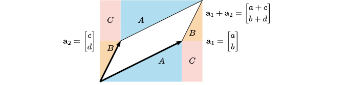
Observe tht \((a+c)(b+d)=ab+cd+ad+bc\) is the area of the rectangle that encloses the parallelepiped spanned by \(\mathbf a_1\), and \(\mathbf a_2\). However, the parallelepiped itself is smaller than the rectangle, and the difference between the two is \(2(A+B+C)=2(\frac{ab}2+\frac{cd}2+bc)\). Therefore, the area of the parallelepiped alone becomes the following.
\[ab+cd+ad+bc-ab-cd-2bc=ad-bc=\left\lvert\det\left(\begin{bmatrix}a&b\\c&d\end{bmatrix}\right)\right\rvert\]This result can be generalized for any \(\mathbf A\in\mathbb R^{n\times n}\), where the absolute value ensures that the determinant provides an unsigned volume. Indeed, by swapping the first and second rows we would have obtained \(\det\left(\begin{bmatrix}\mathbf a_2&\mathbf a_1\end{bmatrix}^T\right)=bc-ad=-\det(\mathbf A)\).
Using the volume analogy, understanding determinants of elementary matrices becomes intuitive, including why \(\det(\mathbf E\mathbf A)=\det(\mathbf E)\det(\mathbf A)\), for each of the possible elementary operations.
Orthogonal matrix
Consider an orthogonal matrix \(\mathbf V\in\mathbb R^{n\times n}\), so that \(\mathbf V\mathbf V^T=\mathbf V^T\mathbf V=\mathbf I_n\). This is due the construction of \(\mathbf V=\begin{bmatrix}\mathbf v_1&\mathbf v_2&\dots&\mathbf v_n\end{bmatrix}\), where \(\mathbf v_i^T\mathbf v_i=1\) and \(\mathbf v_i^T\mathbf v_j=0\), \(i\neq j\). Furthermore, \(\mathbf V\) can be written as follows (where \(\mathbf e_i\) represent the column vectors of \(\mathbf I_n\))
\[\begin{align} \mathbf V &=\begin{bmatrix} \mid&\mid&&\mid\\ \mathbf v_1&\mathbf v_2&\dots&\mathbf v_n\\ \mid&\mid&&\mid \end{bmatrix}=\begin{bmatrix}\mid\\\mathbf v_1\\\mid\end{bmatrix}\begin{bmatrix}1&0&\dots&0\end{bmatrix}+\dots+\begin{bmatrix}\mid\\\mathbf v_n\\\mid\end{bmatrix}\begin{bmatrix}0&0&\dots&1\end{bmatrix}\\ &=\mathbf v_1\mathbf e_1^T+\mathbf v_2\mathbf e_2^T+\dots+\mathbf v_n\mathbf e_n^T=\sum_{i=1}^n\mathbf v_i\mathbf e_i^T \end{align}\]The last relationship is handy if we want to review the nature of \(\mathbf V\mathbf V^T\) (where \(\mathbf e_i^T\mathbf e_i=1\) and \(\mathbf e_i^T\mathbf e_j=0\), \(i\neq j\)).
\[\begin{align} \mathbf I_n=\mathbf V\mathbf V^T &=\left(\sum_{i=1}^n\mathbf v_i\mathbf e_i^T\right)\left(\sum_{j=1}^n\mathbf v_j\mathbf e_j^T\right)^T=\left(\sum_{i=1}^n\mathbf v_i\mathbf e_i^T\right)\left(\sum_{j=1}^n\mathbf e_j\mathbf v_j^T\right)\\ &=\sum_{i=1}^n\sum_{j=1}^n\mathbf v_i\mathbf e_i^T\mathbf e_j\mathbf v_j^T=\sum_{i=1}^n\mathbf v_i\mathbf v_j^T \end{align}\]Spectral theorem for symmetric matrices
Using induction, one can provide some intuitive arguments without going into rigorous derivation. In general, the spectral theorem claims that any symmetric matrix \(\mathbf A\in\mathbb R^{n\times n}\) can be decomposed into \(\mathbf A=\mathbf V\mathbf D\mathbf V^T\), where \(\mathbf V\) is an orthogonal matrix and \(\mathbf D=\text{diag}(\lambda_1,\dots,\lambda_n)\) is a diagonal matrix with \(\lambda_i\) eigenvalues of \(\mathbf A\) on its main diagonal. Notice that \(\mathbf V^T\mathbf A\mathbf V=\mathbf V^T(\mathbf V\mathbf D\mathbf V^T)\mathbf V=\mathbf D\).
Consider \(n=1\), and assume \(\mathbf A=\lambda\), \(\mathbf V=1\) and \(\mathbf D=\lambda\). The relationship is obvious \(\mathbf A=1\lambda1^T\).
Now, consider \(n=2\) and observe as follows, bearing in mind that \(\mathbf v_i\) is the eigenvector associated with eigenvalue \(\lambda_i\), and that for each \(\mathbf v_i\) we have that \(\mathbf v_i^T\mathbf v_i=\lVert\mathbf v_i\rVert_2^2=1\) and \(\mathbf v_i^T\mathbf v_j=0\) if \(i\neq j\).
\[\begin{align} \mathbf V^T\mathbf A\mathbf V&=\begin{bmatrix}\mathbf v_1^T\\\mathbf v_2^T\end{bmatrix}\mathbf A\begin{bmatrix}\mathbf v_1&\mathbf v_2\end{bmatrix} =\begin{bmatrix}\mathbf v_1^T\mathbf A\mathbf v_1&\mathbf v_1^T\mathbf A\mathbf v_2\\\mathbf v_2^T\mathbf A\mathbf v_1&\mathbf v_2^T\mathbf A\mathbf v_2\end{bmatrix}\\ &=\begin{bmatrix}\lambda_1\mathbf v_1^T\mathbf v_1&\lambda_2\mathbf v_1^T\mathbf v_2\\\lambda_1\mathbf v_2^T\mathbf v_1&\lambda_2\mathbf v_2^T\mathbf v_2\end{bmatrix}=\begin{bmatrix}\lambda_1&0\\0&\lambda_2\end{bmatrix}=\mathbf D \end{align}\]Finally, consider \(n>2\) with \(\mathbf V=\begin{bmatrix}\mathbf v_1&\mathbf V_2\end{bmatrix}\), where \(\mathbf V_2\in\mathbb R^{n\times(n-1)}\) and follow the same steps as above, observing that symmetry of \(\mathbf A\) leads to \(\mathbf v_1^T\mathbf A\mathbf V_2=(\mathbf A\mathbf v_1)^T\mathbf V_2=\lambda_1\mathbf v_1^T\mathbf V_2=\mathbf 0_{n-1}^T\).
\[\begin{align} \mathbf V^T\mathbf A\mathbf V&=\begin{bmatrix}\mathbf v_1^T\\\mathbf V_2^T\end{bmatrix}\mathbf A\begin{bmatrix}\mathbf v_1&\mathbf V_2\end{bmatrix} =\begin{bmatrix}\mathbf v_1^T\mathbf A\mathbf v_1&\mathbf v_1^T\mathbf A\mathbf V_2\\\mathbf V_2^T\mathbf A\mathbf v_1&\mathbf V_2^T\mathbf A\mathbf V_2\end{bmatrix}=\begin{bmatrix}\lambda_1&\mathbf 0_{n-1}^T\\\mathbf 0_{n-1}&\mathbf D_2\end{bmatrix}=\mathbf D \end{align}\]Where the relationship \(\mathbf D_2=\text{diag}(\lambda_2,\dots,\lambda_n)=\mathbf V_2^T\mathbf A\mathbf V_2\in\mathbb R^{n-1\times n-1}\) can be proved recursively.
Bearing in mind that \(\mathbf D=\sum_{i=1}^n\lambda_i\mathbf e_i\mathbf e_i^T\), it follows that \(\mathbf A\) can also be expressed as follows.
\[\mathbf A=\mathbf V\left(\sum_{i=1}^n\lambda_i\mathbf e_i\mathbf e_i^T\right)\mathbf V^T=\sum_{i=1}^n\lambda_i(\mathbf V\mathbf e_i)(\mathbf V\mathbf e_i)^T=\sum_{i=1}^n\lambda_i\mathbf v_i\mathbf v_i^T\]Determinant of a symmetric matrix
Consider the characteristic polynomial \(\det(\lambda\mathbf I_n-\mathbf A)\) and observe that if \(\mathbf A\) is symmetric, then the following holds.
\[\begin{align} \det(\lambda\mathbf I_n-\mathbf A) &=\det(\lambda\mathbf V\mathbf I_n\mathbf V^T-\mathbf V\mathbf D\mathbf V^T)=\det(\mathbf V(\lambda\mathbf I_n-\mathbf D)\mathbf V^T)\\ &=\det(\mathbf V)\det(\lambda\mathbf I_n-\mathbf D)\det(\mathbf V^T)=1\cdot\prod_{i=1}^n(\lambda-\lambda_i)\cdot1 \end{align}\]By setting \(\lambda=0\), \(\det(-\mathbf A)=\prod_{i=1}^n(-\lambda_i)\). Analogously, \(\det(\mathbf A)=\prod_{i=1}^n\lambda_i\).
Trace of a symmetric matrix
By definition, \(\text{tr}(\mathbf A)=\sum_{i=1}^n\mathbf e_i^T\mathbf A\mathbf e_i\). If \(\mathbf A=\sum_{i=1}^n\lambda_i\mathbf v_i\mathbf v_i^T\) is symmetric, the following can be derived.
\[\begin{align} \text{tr}(\mathbf A)=\sum_{i=1}^n\mathbf e_i^T\left(\sum_{j=1}^n\lambda_j\mathbf v_j\mathbf v_j^T\right)\mathbf e_i=\sum_{j=1}^n\lambda_j\sum_{i=1}^n(\mathbf e_i^T\mathbf v_j)^2=\sum_{j=1}^n\lambda_j\lVert\mathbf v_j\rVert_2^2=\sum_{j=1}^n\lambda_j \end{align}\]Matrix calculus
If \(f:\mathbb R^d\rightarrow\mathbb R\), with parameter \(\mathbf x=\begin{bmatrix}x_1&\dots&x_d\end{bmatrix}\), the gradient of \(f\) is defined as a column vector \(\nabla_x f\in\mathbb R^d\) that contains partial derivatives with respect to each dimensions on its rows.
\[\nabla_x f(x_1,\dots,x_d)=\begin{bmatrix}\frac\partial{\partial x_1}f\\\vdots\\\frac\partial{\partial x_d}f\end{bmatrix}\]Consider \(\mathbf v=\begin{bmatrix}v_1&\dots&v_d\end{bmatrix}^T\) and \(f(x_1,\dots,x_d)=\mathbf x^T\mathbf v=\sum_{i=1}^dx_iv_i\).
\[\nabla_x(\mathbf x^T\mathbf v)=\begin{bmatrix}\frac\partial{\partial x_1}\sum_{i=1}^dx_iv_i\\\vdots\\\frac\partial{\partial x_d}\sum_{i=1}^dx_iv_i\end{bmatrix}=\begin{bmatrix}v_1\\\vdots\\v_d\end{bmatrix}=\mathbf v\]Note that \(\mathbf x^T\mathbf v\) is a scalar, and is equal to \(\mathbf v^T\mathbf x\). Since the gradient by definition is a column vector in \(d\) dimensions, it follows that \(\nabla_x(\mathbf x^T\mathbf v)=\nabla_x(\mathbf v^T\mathbf x)=\mathbf v\in\mathbb R^d\).
For \(\mathbf A=\begin{bmatrix}\mathbf v_1&\dots&\mathbf v_r\end{bmatrix}\), we have as follows
\[\nabla_x(\mathbf x^T\mathbf A)=\begin{bmatrix}\nabla_x(\mathbf x^T\mathbf v_1)&\dots&\nabla_x(\mathbf x^T\mathbf v_r)\end{bmatrix}=\begin{bmatrix}\mathbf v_1&\dots&\mathbf v_r\end{bmatrix}=\mathbf A\]To remain consistent with the convention that \(\nabla_x(\mathbf x^T\mathbf v)=\nabla_x(\mathbf v^T\mathbf x)=\mathbf v\), we have to consider \(\nabla_x(\mathbf A^T\mathbf x)=\nabla_x(\mathbf x^T\mathbf A)=\mathbf A\). As one may reasonably expect, \(\nabla_x(\mathbf x^T\mathbf I)=\nabla_x(\mathbf I\mathbf x)=\mathbf I\). Finally, for quadratic form we have the following.
\[\nabla_x(\mathbf x^T\mathbf A\mathbf x)=\nabla_x(\mathbf x^T\mathbf A)\mathbf x+\mathbf x^T\mathbf A\nabla_x(\mathbf x)=\mathbf A\mathbf x+\mathbf A^T\mathbf x=(\mathbf A+\mathbf A^T)\mathbf x\]Note that to maintain dimensions consistency, in the above we had to transpose \(\mathbf x^T\mathbf A\). If \(\mathbf A=\mathbf A^T\), then \(\nabla_x(\mathbf x^T\mathbf A\mathbf x)=2\mathbf A\mathbf x\), which is very comforting as it gives an intuitive answer if \(\mathbf A\) were a scalar.