Linear Regression
Linear (or affine) relationship
A relationship between \(x\) and \(y\) is said to be linear if \(y=\beta x\), for some \(\beta\in\mathbb R\). Furthermore, the relationship between \(x\) and \(y\) is affine if \(y=\beta_0+\beta_1x\), for \(\beta_0,\beta_1\in\mathbb R\). Although the term affine implies linearity, for historic reasons linearity is a more widely used term. Indeed, often the affine relationship of the form \(y=\beta_0+\beta_1x=\mathbf x^T\boldsymbol{\beta}\) is still referred to as linear, with \(\mathbf x=\begin{bmatrix}1&x\end{bmatrix}^T\in\mathbb R^2\) and \(\boldsymbol{\beta}=\begin{bmatrix}\beta_0&\beta_1\end{bmatrix}^T\in\mathbb R^2\).
Linear model with noise
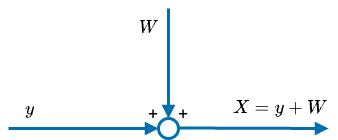
A linear model (LM) reflects a situation where the unknown variable \(y\) is observed indirectly and is affected by noise. The simplest LM is \(X=y+W\), where \(X\) is an observation, \(y\) is the unknown, and \(W\) is the noise, with \(\mathbb E[W]=0\) and \(\text{var}(W)=\sigma^2\). A model so described translates an unknown constant into a r.v. \(X\), s.t. \(\mathbb E[X]=y\) and \(\text{var}(X)=\sigma^2\).
Bayesian statistics models the uncertainty surrounding \(y\) in the form of a prior distribution \(\pi(y)\), s.t. \(\mathbb E[Y]=x_0\) and \(\text{var}(Y)=\sigma_0^2\). Therefore, if \(X=Y+W\) then \(\mathbb E[X]=x_0\) and \(\text{var}(X)=\sigma_0^2+\sigma_i^2\). Upon reading \(X\), we can exploit the Bayes rule and update our prior belief by computing the posterior \(\pi(y\lvert x)\), necessary to derive the LMS estimator \(\hat Y=\mathbb E[Y\lvert X]\). Assuming the distribution of \((X,Y)\) is described by \(f_{XY}(x,y)\), the LMS premises on the existence of a nonzero marginal distribution \(f_X(x)\), the conditional distribution \(f_{Y\lvert X}(y\lvert x)\) and expectation \(\mathbb E[Y\lvert X=x]=\int_{-\infty}^\infty yf_{Y\lvert X}(y\lvert x)dy\).
When the conditional expectations happens to be linear in \(x\), \(\hat Y=\mathbb E[Y\lvert X]\) is also linear in \(X\) and if we collect multiple observations \(X_i=Y+W_i\), the estimator \(\hat Y=\mathbb E[Y\lvert\mathbf X]\) will remain linear in \(\mathbf X=\begin{bmatrix}X_1&\dots&X_n\end{bmatrix}^T\), as far as the underlying (linear) model and the distribution \(W_i\lvert X_i\) maintains the same structure.
LMS with Normal noise
A common example where the LMS estimators is linear in observations is when the LM is affected by Normal noise, that is \(W_i\overset{\text{i.i.d.}}{\sim}\mathcal N(0,\sigma_i^2)\) for \(i=1,\dots,n\). Note that when \(\sigma_i^2=\sigma^2\) then even though \(X_i\) and \(X_j\) are dependent, they will be i.i.d. in the conditional space, \(X_i\lvert Y\overset{\text{i.i.d.}}{\sim}\mathcal N(Y,\sigma^2)\). Also, as \(X_i\) is a sum of independent Normal r.v., it follows that upon the first observation \(X_1\), we can derive that \(Y\lvert X_1\sim\mathcal N(\mu_{Y\lvert X_1},\sigma_{Y\lvert X_1}^2)\), where \(\sigma_{Y\lvert X_1}^2\) is the harmonic mean of \(\sigma_0^2\) and \(\sigma_1^2\), and \(\mu_{Y\lvert X_1}\) is a weighted average of \(x_0\) and \(x_1\).
\[\begin{align} \sigma_{Y\lvert X_1}^2&=\frac1{\frac1{\sigma_0^2}+\frac1{\sigma_1^2}}&\mu_{Y\lvert X_1}&=\frac{\frac1{\sigma_0^2}x_0+\frac1{\sigma_1^2}X_1}{\frac1{\sigma_0^2}+\frac1{\sigma_1^2}}\\ &&&=\sigma_{Y\lvert X_1}^2\left(\frac1{\sigma_0^2}x_0+\frac1{\sigma_1^2}X_1\right) \end{align}\]Notice that with additional observation \(X_2\), the parameters of \(Y\lvert X_1,X_2\sim\mathcal N(\mu_{Y\lvert X_1,X_2},\sigma_{Y\lvert X_1,X_2}^2)\) can be obtained in the same way as above, as if the distribution of \(Y\lvert X_1\) were our new prior.
\[\begin{align} \sigma_{Y\lvert X_1,X_2}^2&=\frac1{\frac1{\sigma_{Y\lvert X_1}^2}+\frac1{\sigma_2^2}}&\mu_{Y\lvert X_1,X_2}&=\sigma_{Y\lvert X_1,X_2}^2\left(\frac1{\sigma_{Y\lvert X_1}^2}\mu_{Y\lvert X_1}+\frac1{\sigma_2^2}X_2\right)\\ &=\frac1{\frac1{\sigma_0^2}+\frac1{\sigma_1^2}+\frac1{\sigma_2^2}}&&=\sigma_{Y\lvert X_1,X_2}^2\left(\frac1{\sigma_0^2}x_0+\frac1{\sigma_1^2}X_1+\frac1{\sigma_2^2}X_2\right) \end{align}\]At this point, the common structure is evident and one can generalize for \(n\) observations.
\[Y\lvert\mathbf X\sim\mathcal N(\mu_{Y\lvert\mathbf X},\sigma_{Y\lvert\mathbf X}^2)=\mathcal N\left(\frac{\frac1{\sigma_0^2}x_0+\sum_{i=1}^n\frac1{\sigma_i^2}X_i}{\frac1{\sigma_0^2}+\sum_{i=1}^n\frac1{\sigma_i^2}},\frac1{\frac1{\sigma_0^2}+\sum_{i=1}^n\frac1{\sigma_i^2}}\right)\]Key conclusions from the above are:
- LMS estimator is \(\hat Y=\mathbb E[Y\lvert\mathbf X]=\mu_{Y\lvert\mathbf X}\) and is the average of observations \(x_i\) (\(x_0\) being treated as an observation), with weights determined by respective variances \(\sigma_i^2\);
- As \(Y\lvert\mathbf X\) is Normal, LMS (or Bayesian) estimator and MAP estimator coincide; and
- \(\text{MSE}(\hat Y)=\mathbb E[\text{var}(Y\lvert\mathbf X)]=\sigma_{Y\lvert\mathbf X}^2\) is constant and does not depend on observations. If some \(\sigma_i^2\) are small, then MSE is also small. Conversely, if all \(\sigma_i\) are large, then MSE is also large.
Note that if \(X_i=a_iY+W_i\), we can simply revise it as \(\tilde X_i=Y+\tilde W_i\), with observations \(\tilde X_i=\frac{X_i}{a_i}\) and noise \(\tilde W_i\sim\mathcal N\left(0,\frac{\sigma_i^2}{a_i^2}\right)\). Last remark is that if \(\sigma_i^2=\sigma^2\), and is constant, then \(\sigma_{Y\lvert\mathbf X}^2=\frac{\sigma^2}n\rightarrow0\), confirming the consistency of the estimator.
Linear LMS (LLMS) estimation
Recall that LMS is the minimizer of \(\text{MSE}(\hat Y)=\mathbb E[\text{var}(Y\lvert\mathbf X)]\). Not always the distribution of \(Y\lvert\mathbf X\) is easy to compute, or unlike in the LM with Normal noise, the LMS may be a non-linear function of observations. However, one could force the estimator to be linear in \(\mathbf X\), at the expense of a higher \(\text{MSE}(\hat Y)\), which is what the linear least mean square (LLMS) tries to accomplish.
Single observation
To restrict an estimator to be linear in \(X\), one could impose it to be \(\hat Y=\beta_0+\beta_1X\), with \(\beta_0\) and \(\beta_1\) s.t. \(\text{MSE}(\hat Y)=\mathbb E[(\hat Y-Y)^2]=\mathbb E[(Y-\hat Y)^2]=\mathbb E[(Y-\beta_0-\beta_1X)^2]\) is still minimized:
- first, notice that \(\text{MSE}(\hat Y)=\mathbb E[((Y-\beta_1X)-\beta_0)^2]\) is minimized at \(\beta_0=\mathbb E[Y-\beta_1X]\). This can be observed by setting \(\frac\partial{\partial\beta_0}\text{MSE}(\hat Y)=0\). Therefore, \(\hat Y=\mathbb E[Y]+\beta_1(X-\mathbb E[X])\);
- second, bearing in mind that \(\mathbb E[((Y-\beta_1X)-\mathbb E[Y-\beta_1X])^2]=\text{var}(Y-\beta_1X)\), which in turn can be expanded as \(\text{var}(Y)+\beta_1^2\text{var}(X)-2\beta_1\text{cov}(Y,X)\), find \(\beta_1=\arg\min_{\beta_1}\text{MSE}(\hat Y)\) by setting \(\frac\partial{\partial\beta_1}\text{MSE}(\hat Y)=0\) and deriving \(\beta_1=\frac{\text{cov}(Y,X)}{\text{var}(X)}\); and
- finally, all pieces together bring us \(\hat Y=\mathbb E[Y]+\frac{\text{cov}(Y,X)}{\text{var}(X)}(X-\mathbb E[X])\).
MSE of LLMS estimator is \(\text{var}(Y)(1-\rho_{YX}^2)\), where \(\rho_{YX}=\frac{\text{cov}(Y,X)}{\sqrt{\text{var}(Y)\text{var}(X)}}\) indicates correlation between \(Y\) and \(X\).
\[\begin{align} \text{MSE}(\hat Y) &=\mathbb E[(\hat Y-Y)^2]\\ &=\mathbb E\left[\left(\mathbb E[Y]+\frac{\text{cov}(Y,X)}{\text{var}(X)}(X-\mathbb E[X])-Y\right)^2\right]\\ &=\mathbb E\left[\left(\frac{\text{cov}(Y,X)}{\text{var}(X)}(X-\mathbb E[X])-(Y-\mathbb E[Y])\right)^2\right]\\ &=\frac{\text{cov}^2(Y,X)}{\text{var}^2(X)}\text{var}(X)+\text{var}(Y)-2\frac{\text{cov}(Y,X)}{\text{var}(X)}\text{cov}(Y,X)\\ &=\text{var}(Y)-\frac{\text{cov}^2(Y,X)}{\text{var}(X)}\\ &=\text{var}(Y)(1-\rho_{Y X}^2) \end{align}\]Main highlights:
- LLMS estimator is linear in observations:
- we do not require complete knowledge of distriutions of \(Y\) and \(X\);
- only means, variances and covariance (or correlation) matter;
- unlike LMS, LLMS could fall outside of the parameter space.
- MSE of the LLMS estimator is driven by covariance (or correlation) as follows:
- if \(\lvert\rho_{YX}\rvert=1\), then \(Y\) has a linear relation to \(X\) and MSE is zero;
- if \(\rho_{YX}=0\), then observations are irrelevant (e.g. the relationship between \(X\) and \(Y\) cannot be described as linear, or \(Y\ind X\)), and MSE is the same as variance of \(Y\).
- if \(\mathbb E[Y\lvert X]\) is linear in \(X\), then LMS and LLMS coincide.
Multiple observations
In case of \(n\) observations of \(X_i\), the only change in the above formula would be that we have to find \(\beta_0\) and \(\boldsymbol{\beta}=\begin{bmatrix}\beta_1&\dots&\beta_n\end{bmatrix}^T\), s.t. \(\hat Y=\beta_0+\boldsymbol{\beta}^T\mathbf X\) minimizes \(\text{MSE}(\hat Y)\). To find elements of \(\boldsymbol{\beta}\), we can follow the same steps we did above.
- set \(\beta_0=\mathbb E[Y]-\boldsymbol{\beta}^T\mathbb[\mathbf X]\), which will result in \(\hat Y=\mathbb E[Y]+\boldsymbol{\beta}^T(\mathbf X-\mathbb E[\mathbf X])\);
- compute \(\beta_i=\frac{\text{cov}(Y,X_i)-\sum_{j\neq i}\beta_j\text{cov}(X_i,X_j)}{\text{var}(X_i)}\) by setting \(\nabla_\beta\text{var}(Y-\boldsymbol{\beta}^T\mathbf X)=\mathbf 0\), bearing in mind the following relation.
LLMS with Normal noise
As we look for an estimator of the form \(\hat Y=\beta_0+\boldsymbol{\beta}^T\mathbf X\), coefficients \(\beta_0=(1-\sum_{i=1}^n\beta_i)x_0\) and \(\beta_i=\frac{\sigma_0^2}{\sigma_0^2+\sigma_i^2}(1-\sum_{j\neq i}\beta_j)\) can be derived by noting that \(\text{cov}(Y,X_i)=\text{cov}(X_i,X_j)=\sigma_0^2\), \(\text{var}(X_i)=\sigma_0^2+\sigma_i^2\) and \(\mathbb E[X_i]=\mathbb E[Y]=x_0\). In particular, by resolving a system of \(n\) equations, we determine the following solution.
\[\begin{align} \beta_0=\frac{\frac1{\sigma_0^2}x_0}{\frac1{\sigma_0^2}+\sum_{j=1}^n\frac1{\sigma_j^2}}&&\beta_i=\frac{\frac1{\sigma_i^2}}{\frac1{\sigma_0^2}+\sum_{j=1}^n\frac1{\sigma_j^2}}&&\hat Y=\frac{\frac1{\sigma_0^2}x_0+\sum_{i=1}^n\frac1{\sigma_i^2} X_i}{\frac1{\sigma_0^2}+\sum_{i=1}^n\frac1{\sigma_i^2}} \end{align}\]Which is exactly as the LMS with Normal noise, and the reason being that LMS was already linear in observations. Notably, the above estimator is valid for any distribution, at the condition that the underlying model is linear, that is \(X_i=Y+W_i\), and noise is uncorrelated with the parameter of interest, or \(Y\ind W_i\). In this case, if means and variances are the same as above, then covariances are \(\text{cov}(Y,X_i)=\text{cov}(Y,Y+W_i)=\sigma_0^2\), and \(\text{cov}(X_i,X_j)=\text{cov}(Y+W_i,Y+W_j)=\sigma_0^2\), which will lead us to the same solution.
Linear regression
The function \(f(x)=\mathbb E[Y\lvert X=x]\) is called regression, and is a fundamental tool used to understand relationships between r.v., and aim at predicting the value of \(Y\) based on the observation of \(X=x\).
At the same time, it is important understanding the limitations of using (linear) regression alone, without some additional tools:
- it may not explain or prove any causal relationship between \(X\) and \(Y\). Linear regression exploits correlation between \(X\) and \(Y\), but correlation is not the same as causation;
- it may not prove if the relationship between \(X\) and \(Y\) is linear. Linearity is an assumption made a priori, and if the data is dense enough around a particular point, it may seem linear;
- it may not capture a functional relationship of the sort \(Y=f(X)\), simply because the choice of covariates \(X\) may not be exhaustive.
In literature, there are many different terms to indicate \(X\) and \(Y\), such as regressor/regressand, or independent/dependent variables. This variety is attributable to historical reasons, as regression is being exploited in diverse fields. While in statistical modelling the two may be referered to as explanatory variable/response, in machine learning they could be indicated as features/target. Finally, in research and experimental design they are commonly indicated as covariates/outcomes.
Note that \((X,Y)\) can be seen as a bivariate r.v., entirely described by \(f_{XY}(x,y)\). Among other things, the joint PDF shows interaction between \(X\) and \(Y\), including if the two are correlated, or independent. In most cases, access to the joint PDF is impracticable, and this is when we settle for less information, such as only the expectation, median or quantile of \(Y\) given \(X=x\). This partial analysis (including linear regression) is much easier with discrete \(X\), in which case conditional expectation, variance and quantiles, take form of sample average, variance and quantiles of \(Y_i\) associated with \(X_i=x\), for which we can apply ME techniques.
To this end, recall that the joint PDF can be split into a marginal PDF, \(f_X(x)=\int_{-\infty}^\infty f_{XY}(x,y)dy\), and conditional PDF, \(f_{Y\lvert X}(y\lvert x)=\frac{f_{XY}(x,y)}{f_X(x)}\), which in turn allows computing various conditional quantities, such as expectation \(\mathbb E[Y\lvert X=x]=\int_{-\infty}^\infty yf_{Y\lvert X}(y\lvert x)dy\) and quantiles \(\int_{-\infty}^{q_\alpha(x)} f_{Y\lvert X}(y\lvert x)dy=1-\alpha\).
Univariate regression
As we saw earlier, we can restrict the regression to be linear in observations, that is \(f(x)=\beta_0+\beta_1 x\) with \(\beta_1=\frac{\text{cov}(X,Y)}{\text{var}(X)}\) and \(\beta_0=\mathbb E[Y]-\beta_1\mathbb E[X]\). However, as far as \(\text{var}(Y\lvert X=x)>0\), there will be noise \(\varepsilon=Y-(\beta_0+\beta_1X)\). By construction, \(\mathbb E[\varepsilon]=0\) and \(\text{cov}(X,\varepsilon)=0\). Furthermore, as we do not have access to the underlying distributions, parameters \(\beta_0\) and \(\beta_1\) can be estimated as follows.
\[\begin{align} \hat\beta_1=\frac{\overline{XY}-\bar X\bar Y}{\overline{X^2}-(\bar X)^2}\xrightarrow{\mathbb P}\frac{\text{cov}(X,Y)}{\text{var}(X)}=\beta_1&&\hat\beta_0=\bar Y-\hat\beta_1\bar X\xrightarrow{\mathbb P}\mathbb E[Y]-\beta_1\mathbb E[X]=\beta_0 \end{align}\]Conceptually, \(Y=\hat\beta_0+\hat\beta_1X+\varepsilon\) is a LM with noise. At this point, it will be reasonable testing if \(\varepsilon\sim\mathcal N(\hat\mu_\varepsilon,\hat\sigma_\varepsilon^2)\) to confirm a linear relationship between \(X\) and \(Y\), using KL or QQ plots. If the test fails, a straight line may not be the best fitting for the model, and one may consider some other types of relationship (e.g., polynomial, exponential, logarithmic, etc.), or consider a more generalized approach.
Multivariate regression
When we collect multiple independent variables, each outcome can be expressed as \(Y_i=\mathbf X_i^T\boldsymbol{\beta}+\varepsilon_i\), with \(\mathbf X_i^T=\begin{bmatrix}1&X_i^{(1)}&\dots&X_i^{(d)}\end{bmatrix}\) and \(\boldsymbol{\beta}=\begin{bmatrix}\beta_0&\beta_1&\dots&\beta_d\end{bmatrix}^T\), s.t. \(\text{cov}(\mathbf X_i,\varepsilon_i)=\mathbf 0_d\). After collecting a sample of size \(n\), observations can be conveniently arranged as follows.
\[\mathbf Y=\begin{bmatrix}Y_1\\\vdots\\Y_n\end{bmatrix}=\begin{bmatrix}1&\mathbf X_i^T\\\vdots\\1&\mathbf X_n^T\end{bmatrix}\begin{bmatrix}\beta_0\\\vdots\\\beta_d\end{bmatrix}+\begin{bmatrix}\varepsilon_1\\\vdots\\\varepsilon_n\end{bmatrix}=\mathbf X\boldsymbol{\beta}+\boldsymbol{\varepsilon}\]Since \(\boldsymbol{\beta}\) is a vector that minimizes \(\mathbb E[\varepsilon^2]\), natural estimator of which is \(\frac1n\lVert\boldsymbol{\varepsilon}\rVert_2^2=\frac1n\lVert\mathbf Y-\mathbf X\boldsymbol{\beta}\rVert_2^2\), then one comes to conclusion that \(\boldsymbol{\beta}\) can be estimated as \(\hat{\boldsymbol{\beta}}=\arg\min_{\boldsymbol{\beta}\in\mathbb R^d}\Vert\mathbf Y-\mathbf X\boldsymbol{\beta}\rVert_2^2\), which means that:
\[\begin{align} \nabla_\beta(\mathbf Y-\mathbf X\hat{\boldsymbol{\beta}})^T(\mathbf Y-\mathbf X\hat{\boldsymbol{\beta}})&=-2(\mathbf X^T\mathbf Y-\mathbf X^T\mathbf X\hat{\boldsymbol{\beta}})=0\\ \implies\mathbf X^T\mathbf X\hat{\boldsymbol{\beta}}&=\mathbf X^T\mathbf Y\\ \hat{\boldsymbol{\beta}}&=(\mathbf X^T\mathbf X)^{-1}\mathbf X^T\mathbf Y\\ \end{align}\]Note that \(\hat{\boldsymbol{\beta}}\) is identifiable if \((\mathbf X^T\mathbf X)\) is invertible, which is achieved if \(\text{rank}(\mathbf X)=d\). If \(d=2\), or \(\mathbf x_i^T=\begin{bmatrix}1&x_i\end{bmatrix}\), this means that we should collect at least two observations, and \(x_1\neq x_2\).
Exponential families
Generalized Linear Models (GLM)
Go back to the syllabi breakdown.
Back-up
Multivariate LM with Normal noise
If \(\mathbf Y=\begin{bmatrix}Y_1&\dots&Y_d\end{bmatrix}^T\sim\mathcal N_d(\begin{bmatrix}x_{01}&\dots&x_{0d}\end{bmatrix}^T,\text{diag}(\sigma_{01}^2,\dots,\sigma_{0d}^2))\) and \(X_i=\mathbf a_i^T\mathbf Y+W_i\), with \(\mathbf a_i=\begin{bmatrix}a_{i1}&\dots&a_{id}\end{bmatrix}^T\), we have that \(X_i\lvert\mathbf Y\sim\mathcal N(\mathbf a_i^T\mathbf Y,\sigma_i^2)\). The good news is that \(\mathbf Y\lvert\mathbf X\) is still Normally distributed, according to \(\mathcal N_d(\mu_{\mathbf Y\lvert\mathbf X},\sigma_{\mathbf Y\lvert\mathbf X}^2)\), and that for any \(j=1,\dots,d\), the posterior of \(Y_j\lvert\mathbf X,\mathbf Y_{k\neq j}\) is Normal with the same structure as above, provided that \(\tilde X_{ij}=\frac{X_i-\sum_{k\neq j}a_{ik}Y_k}{a_{ij}}\) and \(\tilde\sigma_{ij}^2=\frac{\sigma_i^2}{a_{ij}^2}\) for \(i\ge1\).
\[Y_j\lvert\mathbf X,\mathbf Y_{k\neq j}\sim\mathcal N\left(\frac{\frac1{\sigma_{0j}^2}x_{0j}+\sum_{i=1}^n\frac1{\tilde\sigma_{ij}^2}\tilde X_{ij}}{\frac1{\sigma_{0j}^2}+\sum_{i=1}^n\frac1{\tilde\sigma_{ij}^2}},\frac1{\frac1{\sigma_{0j}^2}+\sum_{i=1}^n\frac1{\tilde\sigma_{ij}^2}}\right)\]While glossing over the details, the above can be derived as in the univariate case \(Y\lvert\mathbf X\), by adding one observation at a time. Observe the posterior after a single observation \(X_1\) and isolate \(y_j\).
\[\begin{align} \pi(\mathbf y\lvert X_1)&\propto\pi(\mathbf y)\mathcal L_1(X_1\lvert\mathbf y)=\pi(y_j)\pi(\mathbf y_{k\neq j})\mathcal L_1(X_1\lvert y_j,\mathbf y_{k\neq j})\\ &\propto\exp\left\{-\frac12\left(\frac{y_j-x_{0j}}{\sigma_{0j}}\right)^2\right\}\pi(\mathbf y_{k\neq j})\exp\left\{-\frac12\left(\frac{X_1-\sum_{k\neq j}a_{1k}y_k-a_{1j}y_j}{\sigma_1}\right)^2\right\}\\ &=\exp\left\{-\frac12\left[\left(\frac{y_j-x_{0j}}{\sigma_{0j}}\right)^2+\left(\frac{\tilde X_{1j}-y_j}{\tilde\sigma_{1j}}\right)^2\right]\right\}\pi(\mathbf y_{k\neq j}) \end{align}\]Since the above is another sum of independent Normal r.v., its exponent can be further split as follows.
\[\begin{align} \pi(\mathbf y\lvert X_1) &\propto\exp\left\{-\frac12\left[\left(\frac{y_j-\mu_{Y_j\lvert X_1,\mathbf Y_{k\neq j}}}{\sigma_{Y_j\lvert X_1,\mathbf Y_{k\neq j}}}\right)^2+\left(\frac{X_1-\mu_{X_1\lvert\mathbf Y_{k\neq j}}}{\sigma_{X_1\lvert\mathbf Y_{k\neq j}}}\right)^2\right]\right\}\pi(\mathbf y_{k\neq j})\\ &\propto\pi(y_j\lvert X_1,\mathbf Y_{k\neq j})\mathcal L_1(X_1\lvert\mathbf Y_{k\neq j})\pi(\mathbf y_{k\neq j})\propto\pi(y_j\lvert X_1,\mathbf Y_{k\neq j})\pi(\mathbf y_{k\neq j}\lvert X_1) \end{align}\]Above separation shows that \(Y_j\lvert X_1,\mathbf Y_{k\neq j}\) is Normally distributed, with parameters that are structurally similar to the one obtained in the univariate case, except for some minor adjustments.
\[\begin{align} \sigma_{Y_j\lvert X_1,\mathbf Y_{k\neq j}}^2=\frac1{\frac1{\sigma_{0j}^2}+\frac1{\tilde\sigma_{1j}^2}}&&\mu_{Y_j\lvert X_1,\mathbf Y_{k\neq j}}=\sigma_{Y_j\lvert X_1,\mathbf Y_{k\neq j}}^2\left(\frac1{\sigma_{0j}^2}x_{0j}+\frac1{\tilde\sigma_{1j}^2}\tilde X_{1j}\right) \end{align}\]Iteratively, the above can be generalized for \(n\) observations.
\[\begin{align} \sigma_{Y_j\lvert X_n,\mathbf Y_{k\neq j}}^2=\frac1{\frac1{\sigma_{0j}^2}+\sum_{i=1}^n\frac1{\tilde\sigma_{ij}^2}}&&\mu_{Y_j\lvert X_n,\mathbf Y_{k\neq j}}=\sigma_{Y_j\lvert X_n,\mathbf Y_{k\neq j}}^2\left(\frac1{\sigma_{0j}^2}x_{0j}+\sum_{i=1}^n\frac1{\tilde\sigma_{ij}^2}\tilde X_{ij}\right) \end{align}\]So, in the above derivation we showed that we can split the posterior and segregate individual \(y_j\) to derive respective Bayesian estimators, that is \(\hat Y_j=\mathbb E[Y_j\lvert\mathbf X,\mathbf Y_{k\neq j}]=\mu_{Y_j\lvert\mathbf X,\mathbf Y_{k\neq j}}\).
Remarkably, we would have come to the same conclusion if we derived \(\hat{\mathbf Y}=\arg\max_{\mathbf y\in\mathbb R^d}\pi(\mathbf y\lvert\mathbf X)\), s.t. \(\nabla_y\ln(\pi(\hat{\mathbf y}\lvert\mathbf X))=\mathbf 0\). This can be achieved by taking note of the term in the following term in the exponent of the posterior and setting to zero its partial derivatives, with respect to each \(y_j\).
\[\begin{align} \frac\partial{\partial y_j}\ln(\pi(\mathbf y\lvert\mathbf X)) &=\frac\partial{\partial y_j}\left(-\frac12\sum_{j=1}^d\left(\frac{y_j-x_{0j}}{\sigma_{0j}}\right)^2-\frac12\sum_{i=1}^n\left(\frac{X_i-\sum_{k\neq j}a_{ik}y_k-a_{ij}y_j}{\sigma_i}\right)^2\right)\\ &=-\frac1{\sigma_{0j}^2}(y_j-x_{0j})+\sum_{i=1}^n\frac{a_{ij}}{\sigma_i^2}\left(X_i-\sum_{k\neq j}a_{ik}y_k-a_{ij}y_j\right)\\ &=-y_j\left(\frac1{\sigma_{0j}^2}+\sum_{i=1}^n\frac{a_{ij}^2}{\sigma_i^2}\right)+\left(\frac1{\sigma_{0j}^2}x_{0j}+\sum_{i=1}^n\frac{a_{ij}^2}{\sigma_i^2}\frac{X_i-\sum_{k\neq j}a_{ik}y_k}{a_{ij}}\right)=0\\ \implies\hat Y_j&=\frac{\frac1{\sigma_{0j}^2}x_{0j}+\sum_{i=1}^n\frac1{\tilde\sigma_{ij}^2}\tilde X_{ij}}{\frac1{\sigma_{0j}^2}+\sum_{i=1}^n\frac1{\tilde\sigma_{ij}^2}}=\mu_{Y_j\lvert\mathbf X,\mathbf Y_{k\neq j}} \end{align}\]Note that if \(a_{ij}=0\), then \(\frac1{\tilde\sigma_{ij}^2}=\frac1{\tilde\sigma_{ij}^2}\tilde X_{ij}=0\), and \(x_i\) is irrelevant for the estimation \(Y_j\). Also, \(\hat{\mathbf Y}=\begin{bmatrix}\hat Y_1&\dots&\hat Y_d\end{bmatrix}^T=\begin{bmatrix}\mu_{Y_1\lvert\mathbf X}&\dots&\mu_{Y_d\lvert\mathbf X}\end{bmatrix}^T\), with \(\mu_{Y_j\lvert\mathbf X}\) being the the solutions of a system of \(d\) linear equations.
Considering that LMS derived above is linear in observations, it follows that the LMS estimator coincides with LLMS estimator, both in univariate and multivariate cases.
LMS linear in observation vs LLMS
Since the LLMS is an estimator constrained to be in the form \(\hat Y^{\text{LLMS}}=\beta_0+\beta_1X\), where \(\beta_0\) and \(\beta_1\) are determined in a way to minimize \(\text{MSE}(\hat Y)\), it follows that if an LMS estimator is linear in \(X\), that is \(\hat Y^{\text{LMS}}=a+bX\), then the two estimators necessarily coincide (i.e., \(a=\beta_0\) and \(b=\beta_1\)), because the LMS estimator is by defnition a minimizer of \(\text{MSE}(\hat Y)\).
For illustrative purposes, assume \(Y\sim\text{Unif}(0,1)\) and observations \(X_i\lvert Y\overset{\text{i.i.d.}}{\sim}\text{Ber}(Y)\). Given \(Y\), \(X=\sum_{i=1}^n X_i\) is distributed as \(\text{Bin}(n,Y)\). Since \(\pi(y)=1\), it follows that \(\pi(y\lvert x)\propto y^{x}(1-y)^{n-x}\), or \(Y\lvert X\sim\text{Beta}(1+X,1+n-X)\). Hence, \(\hat Y^{LMS}=\mathbb E[Y\lvert X]=\frac{X+1}{n+2}\), and is linear in \(X\).
Also, note that \(\hat Y^{\text{LLMS}}=\mathbb E[Y]+\frac{\sigma_{XY}}{\sigma_X^2}(X-\mathbb E[X])=\frac{X+1}{n+2}=\hat Y^{\text{LMS}}\), derived observing \(\mathbb E[Y]=\frac12\), \(\text{var}(Y)=\frac1{12}\), \(\mathbb E[Y^2]=\frac13\), \(\mathbb E[X\lvert Y]=nY\), \(\text{var}(X\lvert Y)=nY(1-Y)\), \(\mathbb E[X]=\mathbb E[\mathbb E[X\lvert Y]]=\frac n2\), \(\sigma_{XY}=\href{/2022/01/24/further-topics-on-RV.html#covariance}{\mathbb E[\mathbb E[XY\lvert Y]]-\mathbb E[X]\mathbb E[Y]}=\frac n{12}\), and \(\sigma_X^2=\href{/2022/01/24/further-topics-on-RV.html#total_expectation}{\mathbb E[\text{var}(X\lvert Y)]+\text{var}(\mathbb E[X\lvert Y])}=\frac{n(n+2)}{12}\).
Finally, even though \(\text{bias}(\hat Y)\neq0\), the fact that LLMS coincides with LMS guarantees that the \(\text{MSE}(\hat Y)\) is the minimum attainable, given the linear constraint.
rework
What happens if the underlying model is non-linear? Assume the unknown variable is observed as \(f(\Theta)\) and is still affected by some Normal noise, that is \(X_i=f(\Theta)+W_i\). An intuitive observation would be that \(\Theta=f^{-1}(X_i-W_i)\), which would be equal to \(f^{-1}(X)\) if there were no noise. Therefore, an alternative estimator of the form \(\Theta=af^{-1}(X)+b\) may be considered, which would still be linear in terms of \(a\) and \(b\), with the main drawback that we would be required to compute terms such as \(\text{cov}(\Theta,f^{-1}(X))\) and \(\text{var}(f^{-1}(X))\). The underlying model is called Generalized Linear Model (GLM) and it is something that will be discussed further below.