Introduction to statistics
Motivation
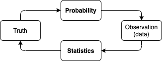
Statistics, Data Science, Machine Learning and Artificial Intelligence, they all use data to get insight and ultimately make decisions. Statistics is at the core of the data processing part, where data comes from a random process.
Accordingly, where probability studies randomness (a way of modeling lack of information) of a phenomenon, which may be completely known (e.g. tossing a coin), statistics focuses on processes where parameters are not known and need to be estimated from data.
Basic inequalities
Fundamental results in statistics are derived from certain inequalities, which attempt to explain probabilities of “extreme events”, using only a bit of information about the underlying distribution (usually expectation and variance).
From the intuition that “if \(X\ge0\) and \(\mathbb E[X]\) is small, then \(X\) is unlikely to be large”, we derive the Markov’s inequality which can be derived from observing that \(\mathbb E[X]\ge\int_{\varepsilon}^\infty\varepsilon f_X(x)dx\).
\[\mathbb P(X\ge\varepsilon)\le\frac{\mathbb E[X]}{\varepsilon},\varepsilon>0\]In the relation above, \(X\) indicates any r.v. Hence, if \(g(X)\) is another, non-negative r.v., an analogous relation can be derived in terms of \(\mathbb E[g(X)]\).
Another intuition, “if the variance is small, then \(X\) is unlikely to be far from the mean”, leads us to the Chebyshev’s inequality, obtained from replacing \(X=(Y-\mathbb E[Y])^2\) in the Markov’s inequality.
\[\mathbb P(\lvert Y-\mathbb E[Y]\lvert\ge\varepsilon)\le\frac{\text{var}(Y)}{\varepsilon^2}\]One may be tempted to think that Chebyshev’s inequality is always tighter than Markov’s inequality; but this is not true and one should evaluate on a case-by-case basis. In general, Markov’s and Chebyshev’s inequalities are too conservative, but are important to prove other claims, including derivation of significantly tigher (exponentially decaying) inequalities. Bear in mind that the above inequalities are an upper bound, therefore there should be no surprise if they can exceed \(1\).
Finally, let \(f(\cdot)\) be a convex and differentiable function. Accordingly, for any \(c\in\mathbb R\) constant, we have that \(f(x)\ge f(c)+f'(c)(x-c)\). If we replace \(x=X\), \(c=\mathbb E[X]\), and apply expectation on both sides of inequality, we obtain the Jensen’s inequality.
\[\mathbb E[f(X)]\ge f(\mathbb E[X])+\cancelto{=0}{f'(\mathbb E[X])(\mathbb E[X]-\mathbb E[X])}\]Common derivations of the Jensen’s inequality include \(\mathbb E[X^{2k}]\ge(\mathbb E[X])^{2k}\) (where \(k=1,2,\dots\)), \(\mathbb E[-\ln(X)]\ge-\ln(\mathbb E[X])\) and \(\mathbb E[e^X]\ge e^{\mathbb E[X]}\).
Weak Law of Large Numbers
According to the weak law of large numbers (WLLN) states that the sample mean \(\bar X_n=\frac{1}{n}\sum_{i=1}^n X_i\) (where \(X_i\overset{\text{i.i.d.}}{\sim}\mathcal P\), with finite \(\mu=\mathbb E[X_i]\) and \(\sigma^2=\text{var}(X_i)\)) converges in probability to the true mean, or \(\bar X_n\xrightarrow[n\rightarrow\infty]{\mathbb P}\mathbb E[X_i]\). To prove, one computes \(\mathbb E[\bar X_n]=\mu\), \(\text{var}(\bar X_n)=\frac{\sigma^2}{n}\), and plugs them into the Chebyshev’s inequality to obtain as follows.
\[\lim_{n\rightarrow\infty}\mathbb P(\lvert\bar X_n-\mu\rvert\ge\varepsilon)\le\frac{\sigma^2}{n\varepsilon^2}=0\]Worth mentioning that according to the strong law of large numbers (SLLN), convergence of the sample mean holds even under a stronger notion of convergence, known as convergence almost surely (or with certain probability), or \(\mathbb P(\lim_{n\rightarrow\infty}\bar X_n=\mu)=1\).
Types of convergences
Denoting \(T_n\) a sequence of r.v. and \(T\) a r.v. (which can also be deterministic), we define the following three convergences.
| Convergence | Notation | Requirement |
|---|---|---|
| Almost surely | \(\displaystyle T_n\xrightarrow[n\rightarrow\infty]{a.s.}T\) | \(\mathbb P(\{\omega:T_n(\omega)\xrightarrow[n\rightarrow\infty]{}T(\omega)\})=1\) |
| In probability | \(\displaystyle T_n\xrightarrow[n\rightarrow\infty]{\mathbb P}T\) | \(\mathbb P(\lvert T_n-T\rvert\ge\varepsilon)\xrightarrow[n\rightarrow\infty]{}0,\forall\varepsilon\gt0\) |
| In distribution | \(\displaystyle T_n\xrightarrow[n\rightarrow\infty]{(d)}T\) | \(\mathbb E[f(T_n)]\xrightarrow[n\rightarrow\infty]{}\mathbb E[f(T)],\forall f\) continuous and bounded or, equivalently \(F_{T_n}(x)\xrightarrow[n\rightarrow\infty]{}F_T(x)\), \(\forall x\) at which \(F_T(x)\) is continuous |
| In \(L^r\) norm | \(T_n\xrightarrow[n\rightarrow\infty]{L^r}\) | \(\displaystyle\lim_{n\rightarrow\infty}\mathbb E[\lvert T_n-T\rvert^r]=0\) |
For ease of notation, note that \(T_n\xrightarrow[n\rightarrow\infty]{a.s./\mathbb P/(d)/L^r}T\) may also be written as \(T_n\xrightarrow{a.s./\mathbb P/(d)/L^r}T\). Follows an overview of mutual implications.
\[\begin{align} T_n\xrightarrow{L^{s>r}}T\implies T_n&\xrightarrow{L^{r\ge1}}T\\ &\Downarrow\\ T_n\xrightarrow{a.s.}T\implies T_n&\xrightarrow{\mathbb P}T\implies T_n\xrightarrow{(d)}T \end{align}\]Difference between “almost surely convergence” and “convergence in probability” is subtle, and is not supposed to be obvious. Eventually, one could refer to a different order of appearance among the limit and probability. Think of the sample mean and rearrange the above requirements as follows.
\[\begin{cases}WLLN:&\displaystyle{\color{red}\lim_{n\rightarrow\infty}}\mathbb P(\lvert\bar X_n-\mu_X\rvert\le\varepsilon)=1\\SLLN:&\displaystyle\mathbb P({\color{red}\lim_{n\rightarrow\infty}}\lvert\bar X_n-\mu_X\rvert=0)=1\end{cases}\]As we increase \(n\): (a) the sample mean \(\bar X_n\) concentrates arbitrarily close around the true mean \(\mu\) in the WLLN; and (b) with certainty, the difference between the two vanishes in the SLLN.
Convergence in \(L^r\) norm for any \(r\ge1\) implies \(T_n\xrightarrow{\mathbb P}T\), as \(\mathbb P(\lvert T_n-T\rvert\ge\varepsilon)\le\frac{\mathbb E[\lvert T_n-T\rvert]}{\varepsilon}\rightarrow0\). So, \(\mathbb E[T_n]\rightarrow t\) implies that \(T_n\xrightarrow{\mathbb P}t\); the converse, however, is not necessarily true.
Convergence properties
According to the continuous mapping theorem (CMT), for \(X_n\xrightarrow{a.s./\mathbb P/(d)}X\) and a continuous \(f(\cdot)\), we have that \(f(X_n)\xrightarrow{a.s./\mathbb P/(d)}f(X)\). Note that CMT can be proved even when \(X_n\) and \(X\) are vectors.
In particular, if we consider a random vector \((X_n,Y_n)\xrightarrow{a.s./\mathbb P}(X,Y)\), and a continuous function \(f(X_n,Y_n)\), we can derive the following relationships.
| \(f(\cdot)\) | Property |
|---|---|
| Addition | \(X_n+Y_n\xrightarrow{a.s./\mathbb P}X+Y\) |
| Multiplication | \(X_nY_n\xrightarrow{a.s./\mathbb P}XY\) |
| Division | \(\displaystyle\frac{X_n}{Y_n}\xrightarrow{a.s./\mathbb P}\frac X Y\), if \(Y_n\neq0\) |
Some partial results can also apply for convergence in distribution. Thanks to Slutsky’s theorem, we have that if \(X_n\xrightarrow{(d)}X\) and \(Y_n\xrightarrow{a.s./\mathbb P}y\), where \(y\in\mathbb R\), then \((X_n,Y_n)\xrightarrow{(d)}(X,y)\). Next we apply CMT, again relying on a continuous \(f(\cdot)\).
| \(f(\cdot)\) | Property |
|---|---|
| Addition | \(X_n+Y_n\xrightarrow{(d)}X+y\) |
| Multiplication | \(X_nY_n\xrightarrow{(d)}Xy\) |
| Division | \(\displaystyle\frac{X_n}{Y_n}\xrightarrow{(d)}\frac X y\), if \(y\neq 0\) |
Central Limit Theorem
The Central Limit Theorem (CLT) states that sum of i.i.d. r.v. tends towards a Normal distribution, as the sample size gets larger and regardless of the population’s distribution. The remarkable thing is that not only this convergence (in distribution) is irrespective of the underlying distribution, but also that the sample size can be moderate (e.g. above 30), especially when the underlying distribution is unimodal and symmetric.
Formally, the CLT states that if \(X_i\overset{\text{i.i.d.}}{\sim}\mathcal P\), with \(\mu_X=\mathbb E[X_i]\) and \(\sigma_X^2=\text{var}(X_i)\), then for the sum \(S_n=\sum_{i=1}^n X_i\) we have that \(S_n\xrightarrow{(d)}\mathcal N(n\mu_X,n\sigma_X^2)\), or \(Z_n=\frac{S_n-n\mu_X}{\sqrt n\sigma_X}\xrightarrow{(d)}\mathcal N(0,1)\). This approximation allows us performing the following queries.
| Query | Application |
|---|---|
| Find \(\mathbb P(S_n\le a)\) | \(\Phi\left(\frac{a-n\mu_X}{\sqrt n\sigma}\right)\) |
| Find \({\color{red} a}\) s.t. \(\mathbb P(S_n\le{\color{red}a})=b\) | \(\displaystyle\frac{ {\color{red}a}-n\mu_X}{\sqrt n\sigma}=\Phi^{-1}(b)\) |
| Find \({\color{red} n}\) s.t. \(\mathbb P(S_{\color{red}n}\le a)=b\) | \(\displaystyle\frac{a-{\color{red} n}\mu_X}{\sqrt{\color{red} n}\sigma}=\Phi^{-1}(b)\) |
An additional application is estimating the probability that a sum of \(n\) copies of \(X_i\) stays below given \(a\). This problem is very similar to describing the probability of \(k\)-th arrival and is formulated as follows.
Assume \(N\) is a r.v. describing the first value for which \(S_N\) exceeds \(a\). At the same time, \(N-1\) is a r.v. describing the last value for which \(S_{N-1}\) is below \(a\). Observing that \(\mathbb P(N>n)=\mathbb P(N-1\ge n)\) we can exploit the arrivals equivalent formulation and derive \(\mathbb P(N>n)=\mathbb P(S_n\le a)\).
CLT and the sample mean
Sample mean is a consistent estimator of the expectation (WLLN) and we know its distribution (CLT). In particular, \(\bar X_n\xrightarrow{(d)}\mathcal N(\mu_X,\frac{\sigma_X^2}{n})\) can be conveniently rewritten in the following two equivalent forms, thanks to standardization.
\[\begin{align} \sqrt{n}(\bar X_n-\mu_X)&\xrightarrow{(d)}\mathcal N(0,\sigma_X^2)\\ \sqrt{n}\frac{(\bar X_n-\mu_X)}{\sigma_X}&\xrightarrow{(d)}\mathcal N(0,1) \end{align}\]Multivariate CLT
In case of a random vector \(\mathbf X\), such that \(\boldsymbol\mu_\mathbf X=\mathbb E[\mathbf X]\) and \(\boldsymbol\Sigma_\mathbf X=\text{cov}(\mathbf X)\), WLLT and CLT can be generalized to a vector of averages \(\bar{\mathbf X}_n\) as follows.
\[\begin{align} \bar{\mathbf X}_n&\xrightarrow{\mathbb P}\boldsymbol\mu_\mathbf X&\href{/2022/02/21/introduction-to-statistics.html#wlln}{\text{(WLLN)}}\\ \sqrt{n}(\bar{\mathbf X}_n-\boldsymbol\mu_{\mathbf X})&\xrightarrow{(d)}\mathcal N_d(\mathbf 0_d,\boldsymbol\Sigma_{\mathbf X})&\href{/2022/02/21/introduction-to-statistics.html#clt}{\text{(CLT)}}\\ \sqrt{n}\boldsymbol\Sigma_{\mathbf X}^{-\frac 1 2}(\bar{\mathbf X}_n-\boldsymbol\mu_{\mathbf X})&\xrightarrow{(d)}\mathcal N_d(\mathbf 0_d,\mathbf I_d) \end{align}\]CLT and the binomial approximation
According to CLT, if \(X_i\overset{\text{i.i.d.}}{\sim}\text{Ber}(p)\) then \(S_n=\sum_{i=1}^n X_i\sim\text{Bin}(n,p)\xrightarrow{(d)}\mathcal N(np,np(1-p))\), which is equivalent to \(\frac{S_n-np}{\sqrt{np(1-p)}}\xrightarrow{(d)}\mathcal N(0,1)\).
Above approximation suffers from Binomial and Normal living in different spaces: where the following holds true in discrete space \(\mathbb P(S_n\lt k+1)=\mathbb P(S_n\le k)\), it may not be true in a continuous space. De Moivre and Laplace addressed this with one-half correction, and we compute \(\mathbb P(S_n\le k+\frac 1 2)\) in the continuous space, which should be equivalent to the former two in the discrete space.
In particular, De Moivre-Laplace correction can be used to approximate binomial PMF as follows.
\[p_{S_n}(k)=\mathbb P\left(k-\frac 1 2\le S_n\le k+\frac 1 2\right)\xrightarrow{(d)}\Phi\left(\frac{k+\frac 1 2-np}{\sqrt{np(1-p)}}\right)-\Phi\left(\frac{k-\frac 1 2-np}{\sqrt{np(1-p)}}\right)\]Try it out in R! (scroll down within the frame to see the result)
Exponentially decaying inequalities
A question may arises concerning the distribution of \(\bar X_n\) when \(n\lt\infty\) and CLT does not apply. We have no reason to assume that \(\bar X_n\) is Normally distributed, however it turns out that we can still make some assumptions regarding the probability of \(\bar X_n\) being far from \(\mu_X=\mathbb E[\bar X_n]\). One option, is using Chebyshev’s inequality to derive \(\mathbb P(\lvert\bar X_n-\mu_X\rvert\ge\varepsilon)\le\frac{\text{var}(\bar X_n)}{\varepsilon^2}=\frac{\sigma_X^2}{n\varepsilon^2}\).
Alternatively, one could use moment generating functions to obtain sharper bound for \(\bar X_n\).
For starters, consider a single r.v. \(X\) and notice that \(\mathbb P(X\ge\varepsilon)=\mathbb P(e^{tX}\ge e^{t\varepsilon})\) for any \(t\gt0\). Thanks to Markov’s inequality, we have that \(\mathbb P(e^{tX}\ge e^{t\varepsilon})\le\mathbb E[e^{tX}]e^{-t\varepsilon}=M_X(t)e^{-t\varepsilon}\) can be made as tight as possible for a suitable \(t\gt0\). Analogously, \(\mathbb P(X\le\varepsilon)\le M_X(t)e^{-t\varepsilon}\) can also be derived for \(t\lt0\). Accordingly, we obtain the basic form of the Chernoff bound.
\[\begin{align}\displaystyle \mathbb P(X\ge\varepsilon)&\le\min_{t\gt0}M_X(t)e^{-t\varepsilon}\\ \mathbb P(X\le\varepsilon)&\le\min_{t\lt0}M_X(t)e^{-t\varepsilon}\\ \end{align}\]Now, replace \(X\) with \(\bar X_n-\mu_X\) and obtain \(\mathbb P(\bar X_n-\mu_X\ge\varepsilon)\le\min_{t\gt0}\left(M_X(t)e^{-t(\varepsilon+\mu_X)}\right)^n\). LHS of the inequality can also be expressed as \(e^{nh(\varepsilon)}\), where \(h(\varepsilon)=\ln\left(\mathbb E[e^{tX_i}]\right)-t(\mu_X+\varepsilon)\) is negative for a suitably small \(t\gt0\). Accordingly, any \(t=\arg\min_{t\gt0}h(\varepsilon)\) will ensure \(h(\varepsilon)\lt0\) and therefore exponential convergence.
Special case is when \(X_i\in[a,b]\) a.s. According to Hoeffding’s lemma \(M_X(t)\le e^{\frac18t^2(b-a)^2}\), which means that \(h(\varepsilon)\le\frac18t^2(b-a)^2-t\varepsilon\), with an upper bound at \(t=\frac{4\varepsilon}{(b-a)^2}\) and therefore as follows.
\[\mathbb P(\bar X_n-\mu_X\ge\varepsilon)\le e^{-\frac{2n\varepsilon^2}{(b-a)^2}}\]Obviously, if the distribution of \(X_i\) is symmetric around \(\mu_X\), then we have the general form of the Hoeffding’s inequality, which holds for any \(n\ge1\).
\[\displaystyle\mathbb P(\lvert\bar X_n-\mu_X\rvert\ge\varepsilon)\le2e^{-\frac{2n\varepsilon^2}{(b-a)^2}}\]Observe that not necessarily Hoeffding’s inequality is tighter than Chebyshev’s inequality, especially for small \(n\).
To give more color to the Chernoff bound, consider \(Z_i\sim\mathcal N(0,\sigma^2)\). In this case, \(M_Z(t)=e^{\frac{t^2}2\sigma^2}\), \(t^\star=\arg\min_{t\gt0}h(\varepsilon)=\frac\varepsilon{\sigma^2}\) and therefore \(h(\varepsilon)=-\frac{\varepsilon^2}{2\sigma^2}\), which means that \(\mathbb P(\bar Z_n\ge\varepsilon)\le e^{-\frac{n\varepsilon^2}{2\sigma^2}}\). In case of Rademacher r.v., for which \(M_R(t)=\mathbb E[e^{tR}]=\sum_{k=0}^\infty\frac{t^{2k}}{(2k)!}\), because \(\mathbb E[R^k]=0\) if \(k\) is odd, and \(\mathbb E[R^k]=1\), if \(k\) is even. Since \((2k)!\ge2^k k!\), then \(M_R(t)\le\sum_{k=0}^\infty\left(\frac{t^2}{2}\right)^k\frac{1}{k!}=e^{\frac{t^2}{2}}\). Using this upper bound, we find that \(t^\star=\arg\min_{t\gt0}h(\varepsilon)=\varepsilon\) and therefore \(\mathbb P(\bar R_n\ge\varepsilon)\le e^{-\frac{n\varepsilon^2}2}\).
Sampling
In real-life experiments, collecting i.i.d. samples may be less trivial as it seems. Clearly, if samples \(X_i\) are not i.i.d., then the normal approximation of \(S_n=\sum_{i=1}^n X_i\) is not guaranteed.
To understand how the Normal approximation can be affected by dependency assume \(M\sim\text{Ber}(\frac 1 2)\) and \(X_i\overset{\text{i.i.d.}}{\sim}\mathcal N(M,1)\). In this example, even though \(X_i\) are i.i.d. the mode of all PDF will strongly depends on the common value of \(M\), which has the same chances to be \(0\) or \(1\). Accordingly, the PDF of \(X\) will not be a Normal, as it will have two modes, around \(0\) and \(1\). This, would have been avoided if \(X_i\overset{\text{i.i.d.}}{\sim}\mathcal N(M_i,1)\), where \(M_i\overset{\text{i.i.d.}}{\sim}\text{Ber}(\frac 1 2)\).
Now, imagine a different case, where \(X_i\sim\text{Ber}(p(t))\), where \(p(t)\) depends on \(t\). If samples \(X_i\) are taken with selected (yet different) \(t\), it may not be possible to assume that observations are identically distributed. The solution in this case is collecting the samples randomly at \(T\), another r.v., so that we could estimate \(\mathbb E[X]=\mathbb E[\mathbb E[X\lvert T]]=\mathbb E[p(T)]\).
From the above, we see that even where \(X_i\) are not i.i.d. (think of polling), we can still make some assumptions about Normal approximation as long as samples collection is done randomly, uniformly and independently, the samples would appear statistically i.i.d.
Go back to the syllabi breakdown.
Back-up
Convergence of a sequence
In this segment it is useful bearing in mind that a sequence is an enumerated collection of elements in which repetitions are allowed and order matters (unlike in a set, where repetitions are not allowed and order does not matter). Formally a sequence can be defined as a function from natural numbers (the position of elements in the sequence) to the elements at each position.
A sequence \(x_n\) is said to converge to \(x\) if for any \(\varepsilon>0\), there exists \(N\) s.t. \(\forall n\ge N, \lvert x_n-x\rvert\le\varepsilon\). Common notation to indicate convergence is \(x_n\xrightarrow[n\rightarrow\infty]{}x\), or simply \(x_n\rightarrow x\).
Observe that if \(x_n\rightarrow x\) and \(y_n\rightarrow y\), then \(x_n+y_n\rightarrow x+y\). To prove this, assume that \(\exists N,M\) for which \(\forall n\ge N\implies\lvert x_n-x\rvert\lt\frac\varepsilon2\) and \(\forall n\ge M\implies\lvert y_n-y\rvert\lt\frac\varepsilon2\). This means that \(\forall n\ge\max\{N,M\}\) we have that \(\lvert x_n+y_n-(x+y)\rvert\le\vert x_n-x\rvert+\lvert y_n-y\rvert\lt\varepsilon\).
Moment generating function
The moment generating function (MGF) is a function that becomes handy for the computation of the first \(m_1,\dots,m_d\) moments. MGF is defined as \(M_X(t)=\mathbb E[e^{tX}]\). Bearing in mind Taylor expansion of \(e^x=\sum_{i=1}^\infty\frac{x^i}{i!}\), it follows that \(M_X(t)=\sum_{i=1}^\infty\frac{t^i}{i!}\mathbb E[X^i]\) and, in particular, that \(\frac{\partial^k}{\partial t^k}M_X(0)=\mathbb E[X^k]\), or \(k\)-th moment of r.v. \(X\).
Properties of MGF include linear transformations, \(M_Y(t)=e^{\beta t}M_X(\alpha t)\) if \(Y=\alpha X+\beta\), and linear combination of independent r.v., \(M_{X+Y}(t)=M_X(t)M_Y(t)\) if \(X\ind Y\).
\[\begin{align} M_X(t)=\sum_x e^{tx}p_X(x)&&M_X(t)=\int_{-\infty}^\infty e^{tx}f_X(x)dx\\ \text{(discrete r.v.)}&&\text{(continuous r.v.)} \end{align}\]Few examples of MGF for basic discrete and continuous r.v.
| Distribution | \(M_X(t)\) |
|---|---|
| Constant \(c\) | \(e^{tc}\) |
| Bernoulli with parameter \(p\) | \(1-p+e^tp\) |
| Binomial with parameters \((k,p)\) | \((1-p+e^tp)^k\) |
| Geometric with parameter \(p\) | \(\displaystyle\frac{e^tp}{1-e^t(1-p)}\) where \(t\lt-\ln(1-p)\) |
| Pascal with parameters \((k,p)\) | \(\displaystyle\left(\frac{e^tp}{1-e^t(1-p)}\right)^k\) where \(t\lt-\ln(1-p)\) |
| Poisson with parameter \(\lambda\) | \(e^{\lambda(e^t-1)}\) |
| Discrete uniform over \([a,b]\) | \(\displaystyle\frac{e^{ta}}{n}\frac{1-e^{tn}}{1-e^t}\) where \(n=b-a+1\) |
| Continuous uniform over \([a,b]\) | \(\displaystyle\frac{e^{tb}-e^{ta}}{\theta t}\) where \(\theta=b-a\) |
| Exponential with parameter \(\lambda\) | \(\displaystyle\frac\lambda{\lambda-t}\) where \(t\lt\lambda\) |
| Erlang with parameters \((k,\lambda)\) | \(\displaystyle\left(\frac\lambda{\lambda-t}\right)^k\) where \(t\lt\lambda\) |
| Gamma with parameters \((\alpha,\beta)\) | \(\displaystyle\left(\frac{\beta}{\beta-t}\right)^\alpha\) where \(t\lt\beta\) |
| Normal with parameters \((\mu,\sigma^2)\) | \(e^{\mu t+\frac12\sigma^2t^2}\) |
As for the derivation of Binomial, Pascal (or Negative Binomial), Erlang and even Gamma, consider that \(M_{X_1+\dots+X_n}(t)=(M_X(t))^n\) where \(X_i\) are \(n\) i.i.d. r.v., therefore their derivation is immediate from Bernoulli, Geometric and Exponential MGFs.
\[\begin{align} M_{X_1+\dots+X_n}(t) &=\int_{-\infty}^\infty\dots\int_{-\infty}^\infty e^{t(X_1+\dots+X_n)}f_{X_1,\dots,X_n}(x_1,\dots,x_n)dx_1\dots dx_n\\ &=\left(\int_{-\infty}^\infty e^{tX_1}f_{X_1}(x_1)dx_1\right)\dots\left(\int_{-\infty}^\infty e^{tX_n}f_{X_n}(x_n)dx_n\right)\\ &=\left(\int_{-\infty}^\infty e^{tX}f_{X}(x)dx\right)^n=\left(M_X(t)\right)^n \end{align}\]Another useful tool is the following Taylor’s expansion of the MFG, for any sufficiently small \(t\).
\[\begin{align} M_X(t) &=M_X(0)+\frac\partial{\partial t}M_X(0)t+\frac12\frac{\partial^2}{\partial t^2}M_X(0)t^2+O(t^3)\\ &\approx1+\mathbb E[X]t+\frac12\mathbb E[X^2]t^2=1+\mu_Xt+\frac12\sigma_X^2t^2 \end{align}\]The above approximation simplifies further when \(\mathbb E[X]=0\), in which case \(M_X(t)\approx1+\frac12\sigma_X^2t^2\).
Final remark is that if \(M_X(t)=M_Y(t)\) for all \(t\) in the neighborhood of \(0\), then \(F_X(u)=F_Y(u)\) for all \(u\). Considering that the Maclaurin expansion of the MGF, \(M_X(t)=1+\mathbb E[X]+\frac12t^2\mathbb E[X^2]+O(t^3)\), highlights that the MGF incapsulates all moments of \(X\), then if \(M_X(t)=M_Y(t)\), for any \(t\) near \(0\) we have that \(\mathbb E[X^i]=\mathbb E[Y^i]\), for any \(i\).
Accordingly, if \(X_n\) is a sequence of r.v. and \(\lim_{n\rightarrow\infty}M_{X_n}(t)=M_Y(t)\) for all \(t\) in the neighborhood of \(0\), then \(\lim_{n\rightarrow\infty}F_{X_n}(u)=F_Y(u)\) for all \(u\). For instance, consider \(X_n\sim\text{Bin}(n,p)\), where \(np=\lambda\).
\[M_{X_n}(t)=(1-p+e^tp)^n=\left(1+\frac{\lambda(e^t-1)}{n}\right)^n\rightarrow e^{\lambda(e^t-1)}=M_Y(t)\]Since \(Y\sim\text{Pois}(\lambda)\), it follows that for a given \(\lambda=np\), Binomial converges to a Poisson as \(n\rightarrow\infty\).
Lindeberg–Lévy Central Limit Theorem
The CLT claims that for any sequence \(X_i\overset{\text{i.i.d.}}{\sim}\mathcal P\), with \(\mathbb E[X]=\mu\lt\infty\) and \(\text{var}(X)=\sigma^2\lt\infty\), then \(\frac{S_n-n\mu}{\sqrt n \sigma}\xrightarrow{(d)}\mathcal N(0,1)\), where \(S_n=\sum_{i=1}^n X_i\).
Since \(\frac{S_n-n\mu}{\sqrt n\sigma}=\frac1{\sqrt n\sigma}\sum_{i=1}^n(X_i-\mu)\), then \(M_{S_n}(t)=\mathbb E\left[e^{t\frac1{\sqrt n\sigma}\sum_{i=1}^n(X_i-\mu)}\right]=\left(M_{X-\mu}\left(\frac t{\sqrt n\sigma}\right)\right)^n\). Also, as \(\mathbb E[X-\mu]=0\), by Taylor’s expansion we have that \(M_{X-\mu}\left(\frac t{\sqrt n\sigma}\right)\approx1+\frac{t^2}{2n}\). In conclusion, \(M_{S_n}(t)\approx\left(1+\frac{t^2}{2n}\right)^n\rightarrow e^{\frac12t^2}\), which is exactly the MGF of \(\mathcal N(0,1)\).
Aside from the exceptional generality of the CLT, it is important to bear in mind that CLT will not work with r.v. with undefined moments, such as Cauchy r.v.
Hoeffding’s lemma
Observe that \(e^{tx}\le\left(\frac{b-x}{b-a}\right)e^{ta}+\left(\frac{x-a}{b-a}\right)e^{tb}\) due to convexity of the exponential function. If we replace \(x=X\) and compute expectation on both sides of the inequality we have the following relation.
\[\mathbb E[e^{tX}]\le\left(\frac{b-\mathbb E[X]}{b-a}\right)e^{ta}+\left(\frac{\mathbb E[X]-a}{b-a}\right)e^{tb}\]Assuming for simplicity that \(\mathbb E[X]=0\), and setting \(p=-\frac{a}{b-a}\), the above can be rewritten as:
\[\begin{align}\mathbb E[e^{tX}]&\le e^{ta}(1-p+pe^{t(b-a)})&\text{replace $t(b-a)=u$}\\ &=e^{ta}(1-p+pe^{u})&\text{replace $ta=-up$}\\ &=e^{\ln(1-p+pe^u)-up}=e^{\varphi(u)}\end{align}\]By Taylor’s expansion, \(\varphi(u)=\varphi(0)+\varphi'(0)u+\frac 1 2 \varphi''(0)u^2+O(u^3)\), and one can verify that \(\varphi(u)=\varphi'(u)=0\) and \(\varphi''(0)=p(1-p)\le\frac 1 4\), because \(0\le p\le1\). This means that \(\varphi(u)\le\frac 1 8u^2\) and therefore:
\[\mathbb E[e^{tX}]\le e^{\frac 1 8 t^2(b-a)^2}\]If we drop our assumption that \(\mathbb E[X]=0\), the above inequality still holds for the first centered moment.
\[\mathbb E[e^{t(X-\mathbb E[X])}]\le e^{\frac 1 8 t^2(b-a)^2}\]